Loading video…


 19 Concepts
 95 views

Video Summary: Line Integrals in the Plane Explained
How do engineers calculate the exact surface area of a curved wall at a landmark like the Gateway Arch in St. Louis? Line integrals in the plane make it possible. This concept allows you to integrate a function along a curved path, not just a straight line, by breaking the curve into infinitely thin strips and summing their contributions. Line Integrals in the Plane Explained shows how parametric equations and Riemann sums combine into a powerful tool. Watch the full video on JoVE Coach to master this concept with expert-led visuals and step-by-step explanations.
Standard integrals measure area under a curve on a flat x-axis. But what if the path itself is curved through two-dimensional space? That is exactly what Line Integrals in the Plane address. Instead of integrating over a fixed interval on the x-axis, you integrate a function f(x, y) over a curve C that winds through the xy-plane. This generalization is one of the most important ideas in multivariable calculus and forms the backbone of vector calculus courses taught at universities across the United States.
A line integral begins with a parametric representation of the curve. The coordinates x and y are both written as functions of a single parameter t, so the curve is described as (x(t), y(t)) for t ranging from a to b. As t increases, a point traces the entire path from start to finish.
The key ingredient connecting the parameter to geometry is the arc length element, written as ds. In plain-text form:
ds = sqrt( (dx/dt)^2 + (dy/dt)^2 ) * dt
This expression measures how much actual distance along the curve corresponds to a tiny change in t. Substituting it into the integral transforms a two-dimensional problem into a single-variable integral that standard calculus techniques can solve. This substitution step is tested regularly in AP Calculus BC free-response questions and in college midterms covering multivariable calculus.
The derivation of a line integral mirrors the logic students already know from basic calculus. Divide the curve into n small segments. On each segment, approximate the function value as roughly constant and multiply it by the small arc length of that segment. This gives one thin rectangular strip of area (or work, or mass, depending on context). Summing all strips produces a Riemann sum. As n approaches infinity and each strip becomes infinitesimally narrow, the sum converges to the definite integral:
Integral over C of f(x, y) ds = Integral from a to b of f(x(t), y(t)) * sqrt( (dx/dt)^2 + (dy/dt)^2 ) dt
This formula is the workhorse of the topic. It applies whether f(x, y) represents a physical height, a material density, or a scalar potential, making it broadly useful in structural engineering, fluid mechanics, and even medical imaging research conducted at institutions like MIT and Johns Hopkins.
Line integrals in the plane are not an isolated technique, they are the foundation for several major theorems in vector calculus. Green's theorem relates a line integral around a closed curve in the plane to a double integral over the enclosed region, linking boundary behavior to interior properties. This theorem is widely applied in fluid dynamics to compute circulation and flux.
Stokes' theorem generalizes this idea to three dimensions by connecting a line integral around a closed loop to a surface integral involving the curl of a vector field. The divergence theorem similarly connects surface integrals to volume integrals. Understanding the physical meaning of divergence, how much a vector field spreads outward from a point, becomes natural once students are comfortable with the line integral framework underneath it.
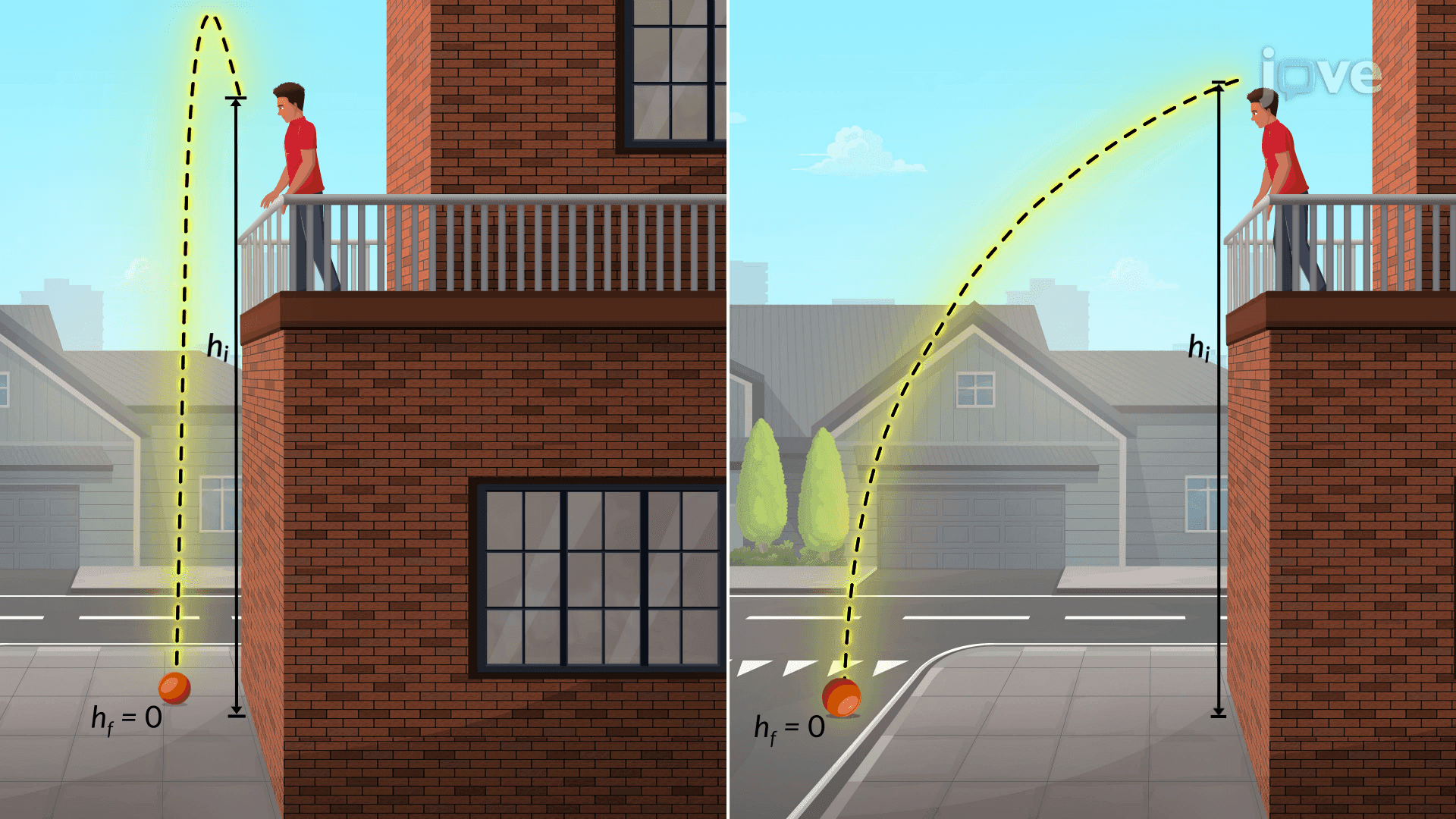
A special case worth mastering is the conservative vector field: when a vector field F equals the gradient of some scalar potential function, the line integral between two points is path-independent. This concept appears on AP Physics C exams and in college-level electromagnetism courses when students calculate electric potential energy between charged particles.
Related Micro-courses