Loading video…

 24 Concepts
 92 views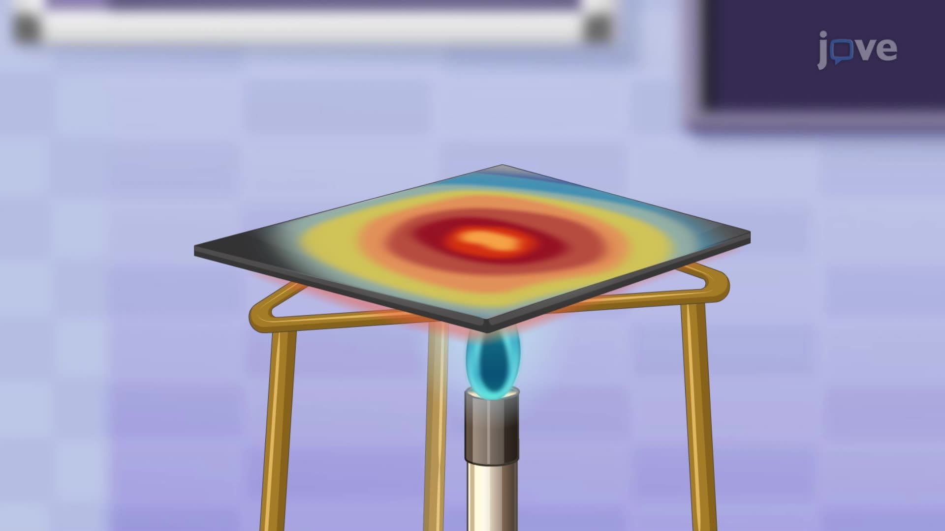

Video Summary: What are Limits of Multivariable Functions
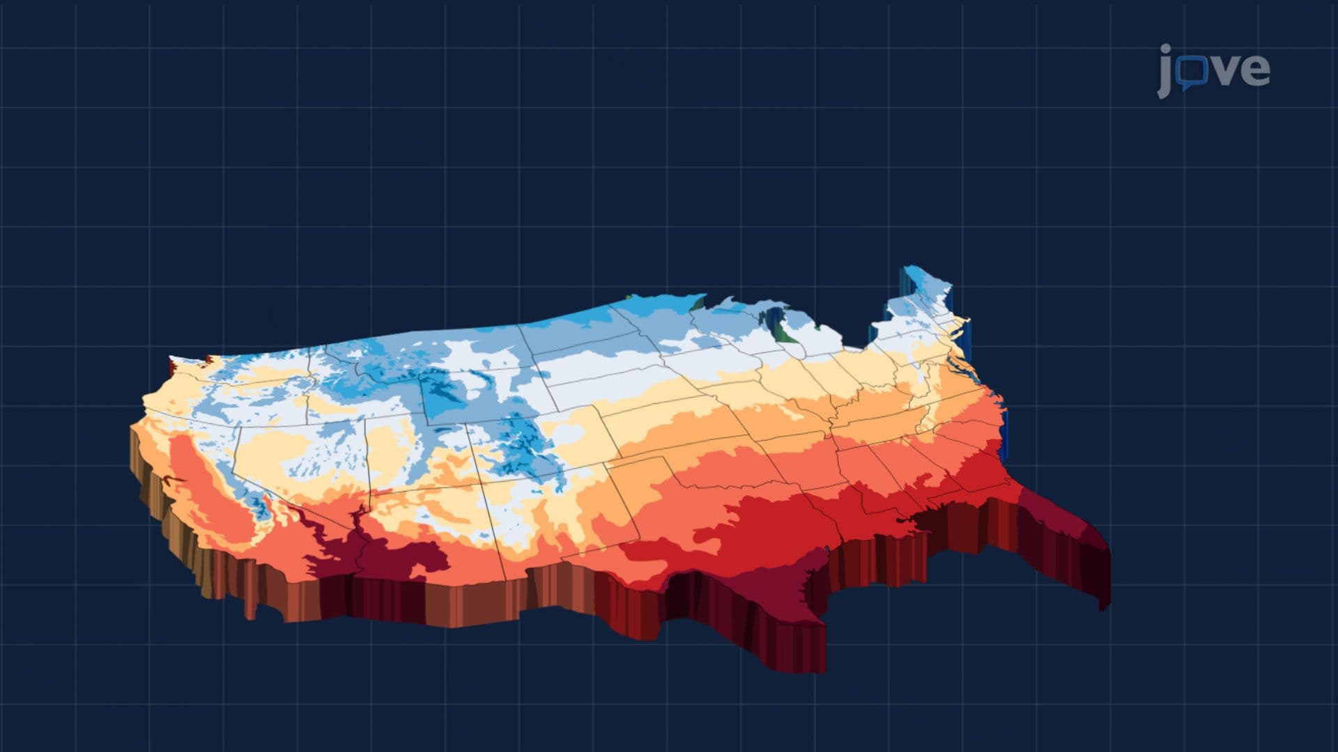
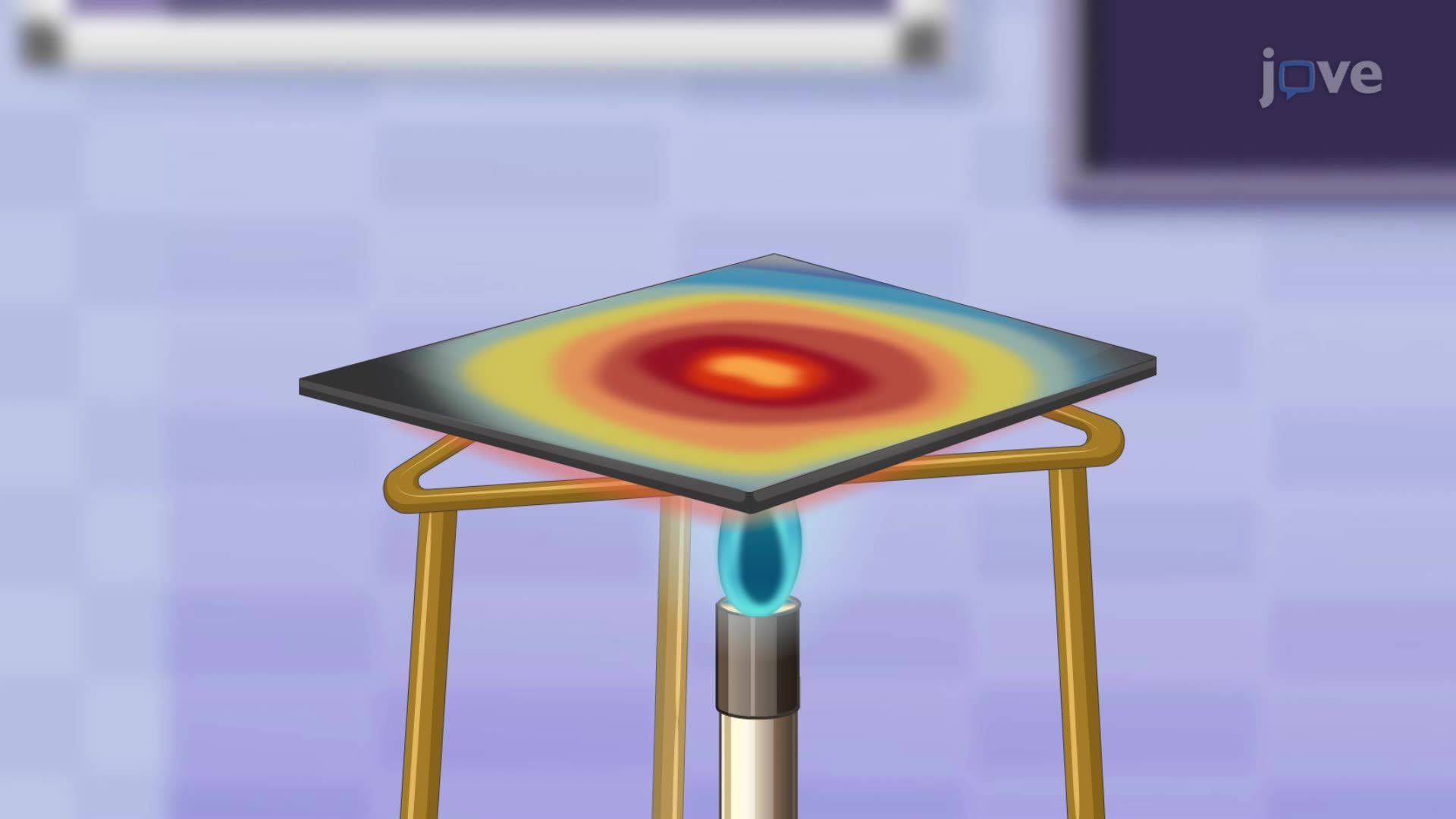
Did you know that modeling heat distribution across a NASA spacecraft's surface requires understanding how temperature approaches a single value from infinitely many directions? That's exactly what the limits of multivariable functions basics reveal. The limits of multivariable functions concept extends single-variable limits into two or more dimensions, using epsilon-delta logic to confirm a function reaches one consistent value from every possible path. Watch the full video on JoVE Coach to master this concept with expert-led visuals and step-by-step explanations.
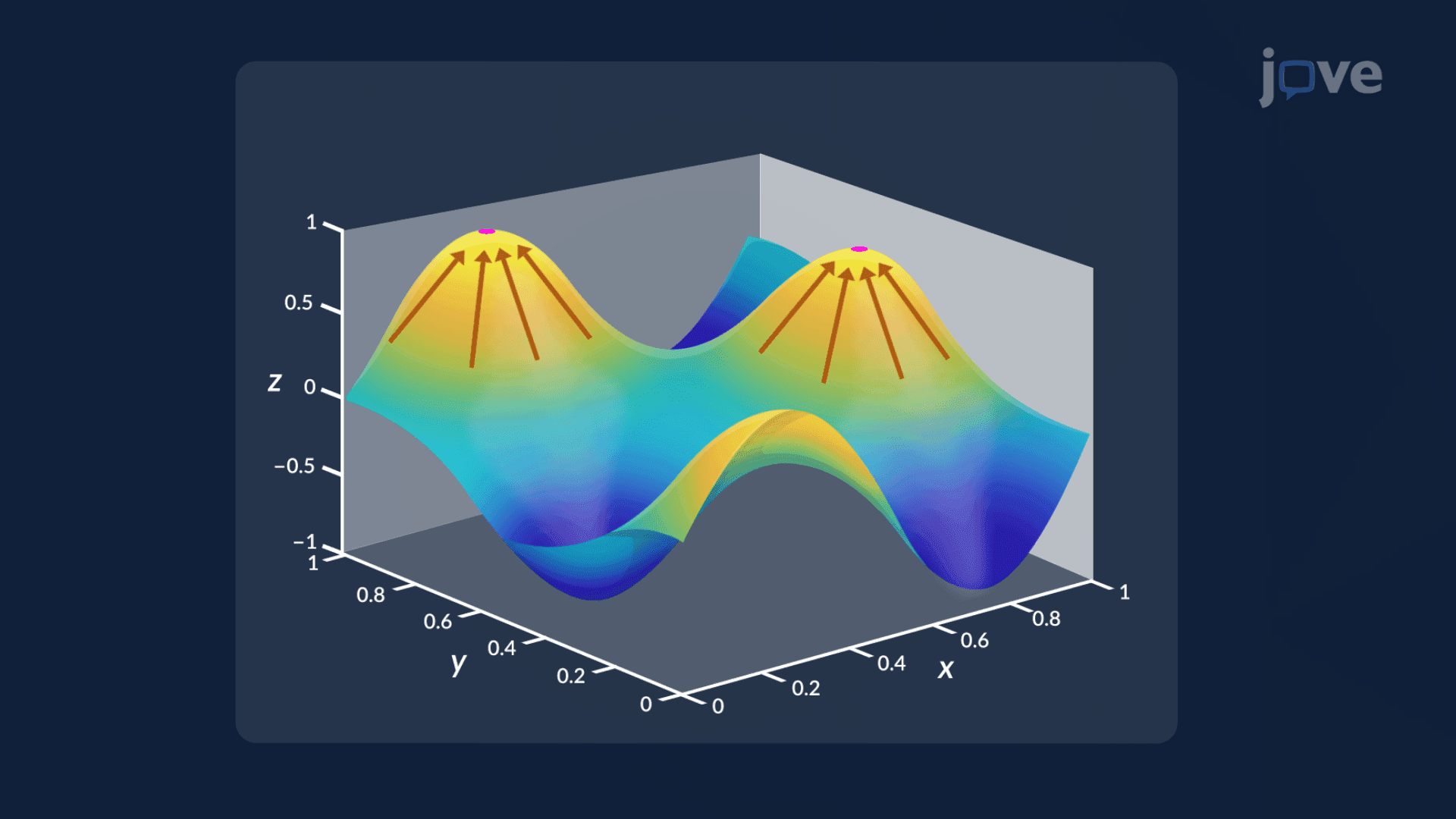
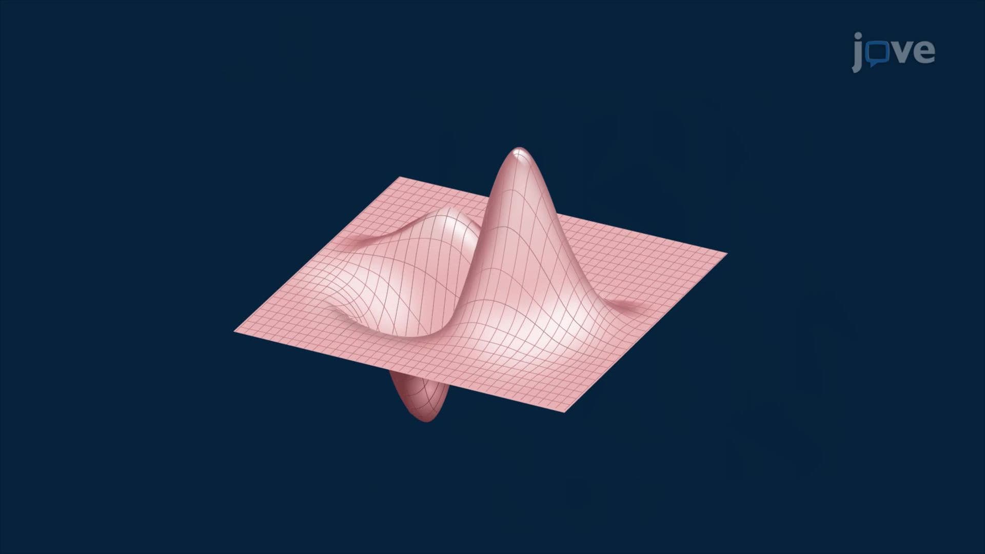
In single-variable calculus, a limit asks: what value does f(x) approach as x gets close to some number? The idea behind limits of multivariable functions extends that question into higher dimensions. For a function f(x, y), a limit L exists only if the function approaches that exact same value from *every conceivable direction*, not just left and right, but along infinitely many paths converging on a single point (a, b) in the xy-plane. This is a stricter, more powerful condition, and it underpins nearly everything in multivariable calculus.
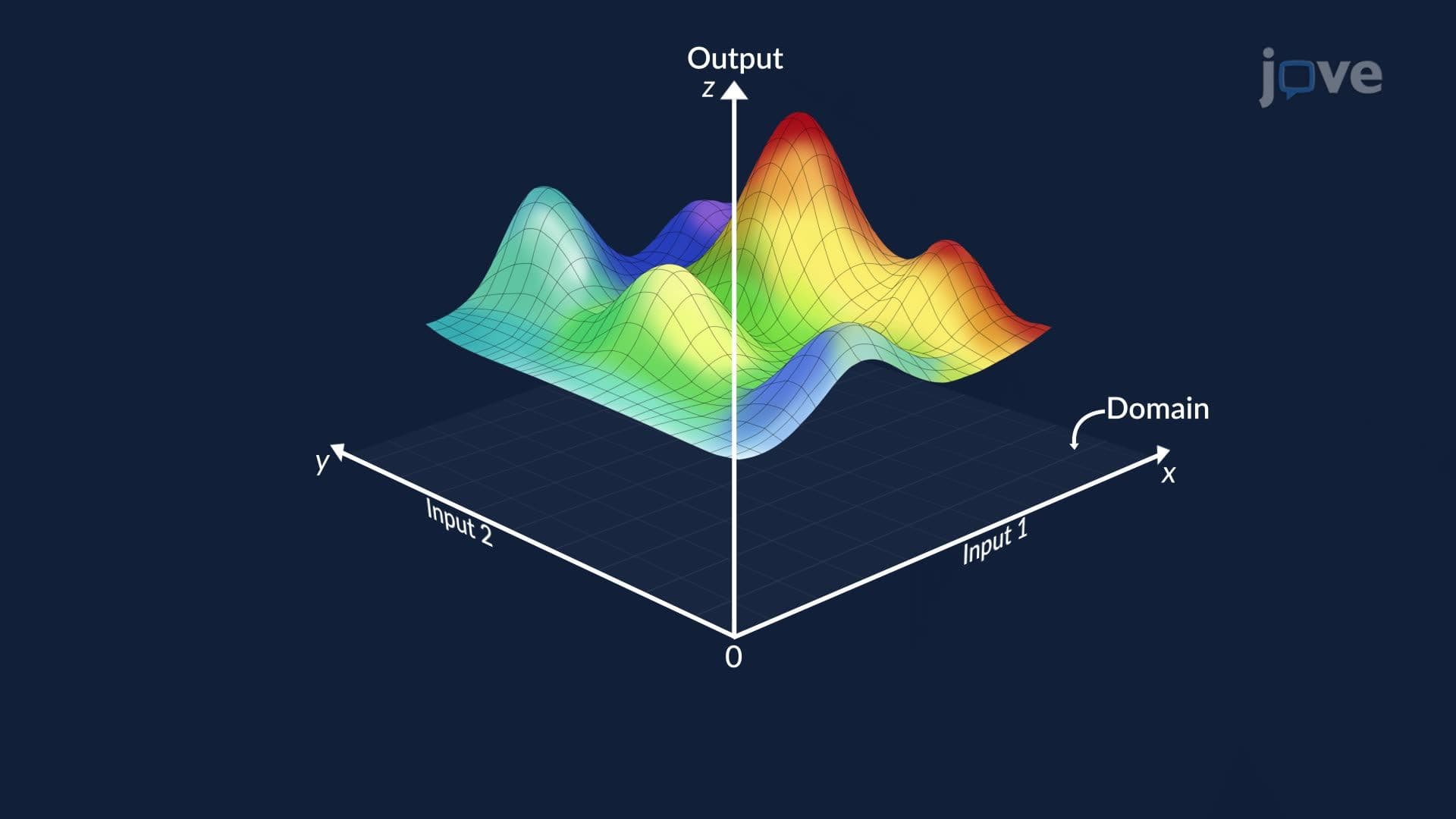
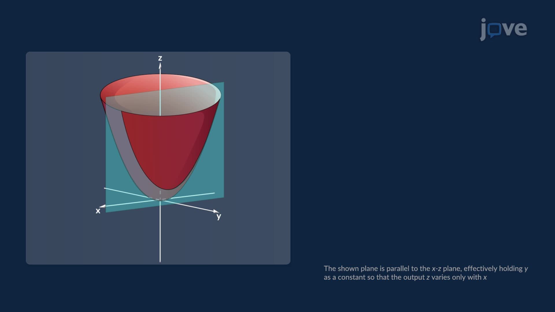
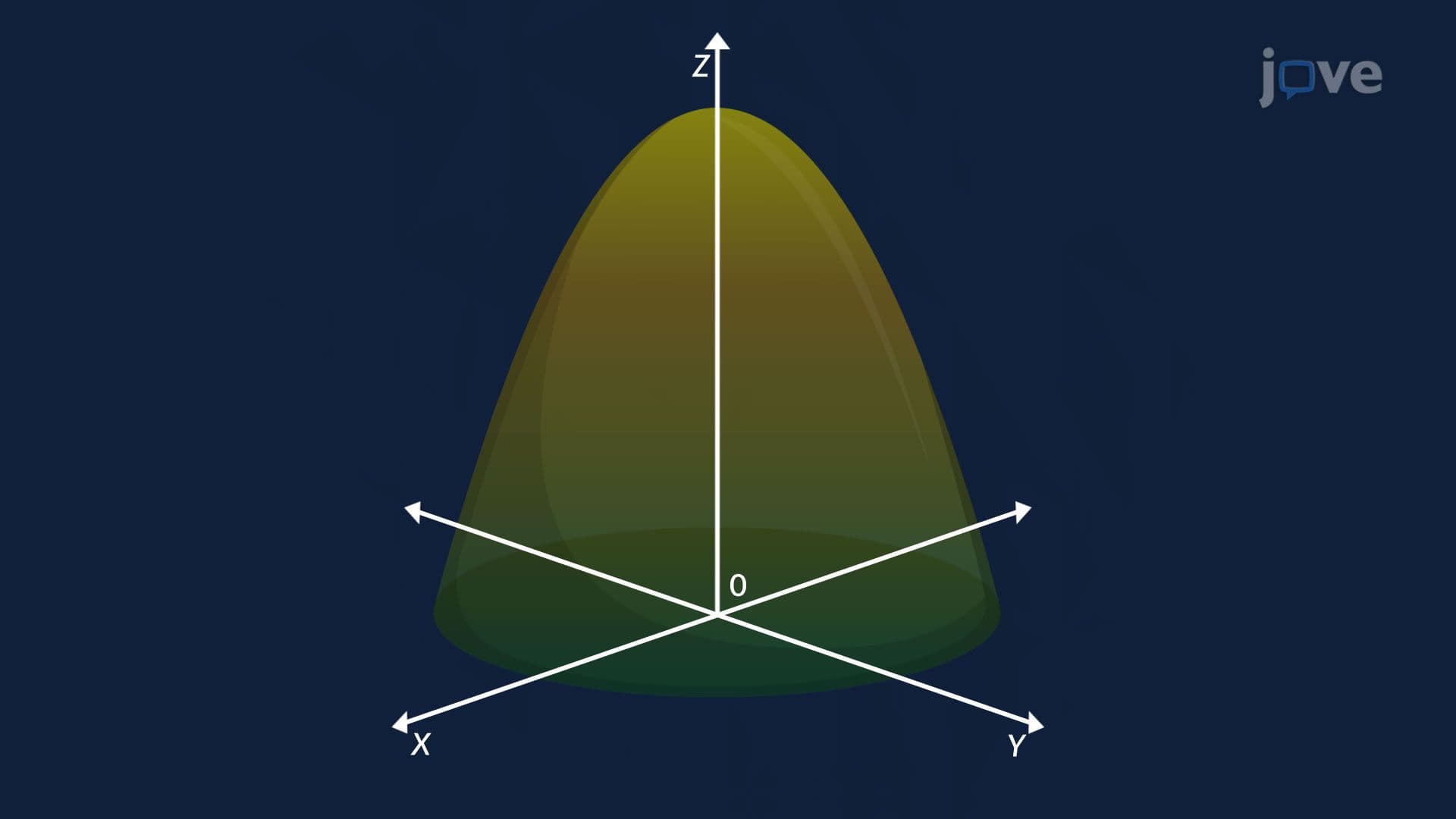
The formal epsilon-delta definition translates naturally from single-variable calculus but gains geometric richness in two dimensions. In 2D, the "delta neighborhood" is no longer an interval on a number line, it becomes a *disk* centered at (a, b) in the xy-plane. For any small positive epsilon (a margin of error around L on the vertical z-axis), there must exist a corresponding delta such that every point (x, y) inside that delta-disk produces an output f(x, y) within epsilon of L.
Think of it like zooming in on a topographic map of a mountain. If every trail you could possibly hike toward a summit converges to the same elevation, the limit exists at that peak. If different trails lead to different heights, the limit does not exist, a critical distinction tested heavily in college-level multivariable calculus courses at universities like MIT, Stanford, and across the UC system.
The biggest challenge students face with limits of multivariable functions explained is the path-dependency problem. Because a point in the xy-plane can be approached along straight lines, parabolas, spirals, or any continuous curve, you must verify consistency across *all* paths, not just a few.
A standard exam technique is to test two straight-line paths first (for example, y = 0 and y = x). If these yield different values, the limit definitively does not exist. However, if both paths give the same value, that is *not* proof the limit exists, you must apply more rigorous methods such as the squeeze theorem or the formal epsilon-delta argument.
This concept appears prominently on AP Calculus BC extensions and is a core topic in university Calculus III (Multivariable Calculus) courses, often appearing on midterms and final exams within the first unit.
The real-world stakes of understanding limits of multivariable functions are significant. Consider a materials engineer at Boeing analyzing thermal stress on an aircraft wing. Temperature at any interior point is modeled as a function of two spatial variables. Confirming that the temperature limit at a critical coordinate is consistent, regardless of the direction of heat flow, allows engineers to certify predictable, safe material behavior.
Similarly, in fluid dynamics, pressure fields modeled as P(x, y) must demonstrate consistent limiting behavior near boundary points to validate computational simulations. These same principles connect directly to directional derivatives, the gradient of a function, and eventually tangent planes, all of which depend on the existence and value of multivariable limits at specific points. Students studying for college midterms will find that mastering this foundational concept makes topics like chain rule for partial derivatives, higher-order partial derivatives, and maximum and minimum values of functions of two variables significantly more approachable.
Related Micro-courses