Loading subject page…

91 views

Video Summary: What are Linear Approximations
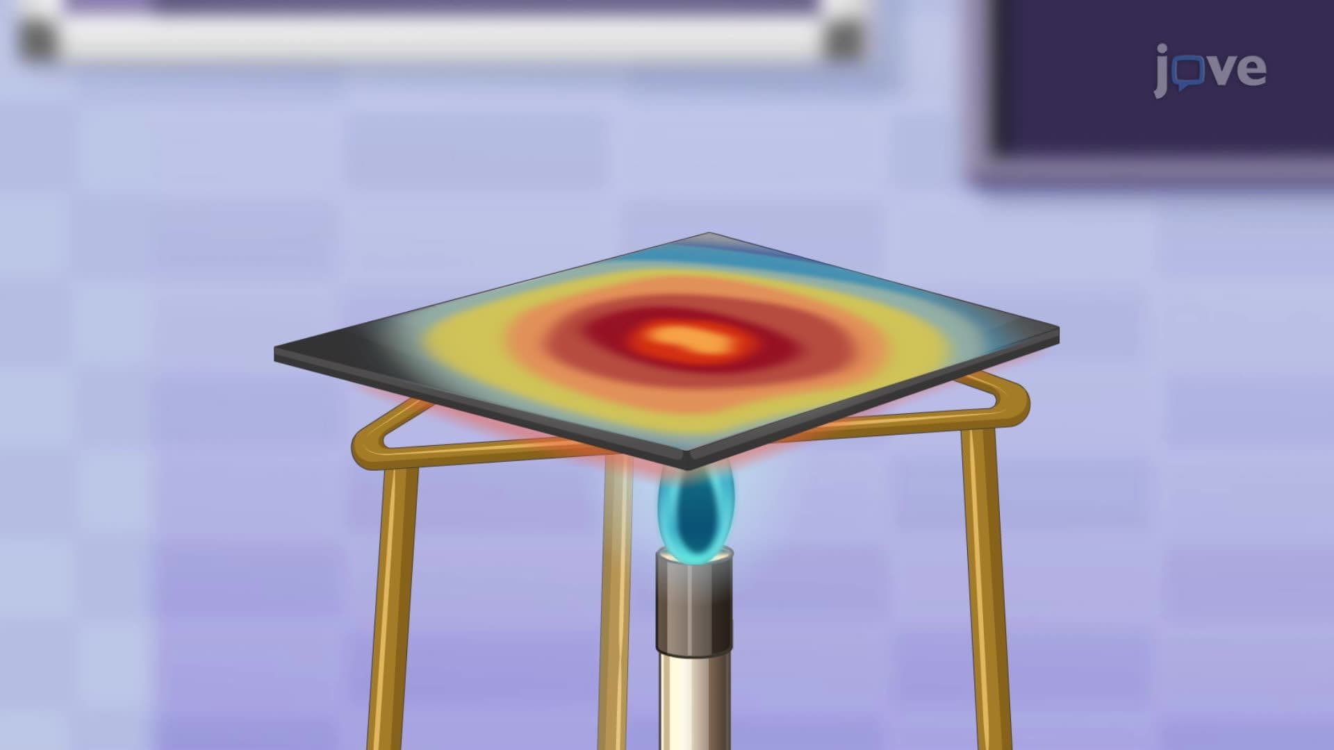
Ever wonder how scientists estimate air pollution levels between monitoring stations without running new measurements? Linear approximations make that possible. This concept in multivariable calculus uses a tangent plane to estimate values of a complex surface near a known point, like predicting pollution concentration near a Chicago monitoring station. Watch the full video on JoVE Coach to master this concept with expert-led visuals and step-by-step explanations.
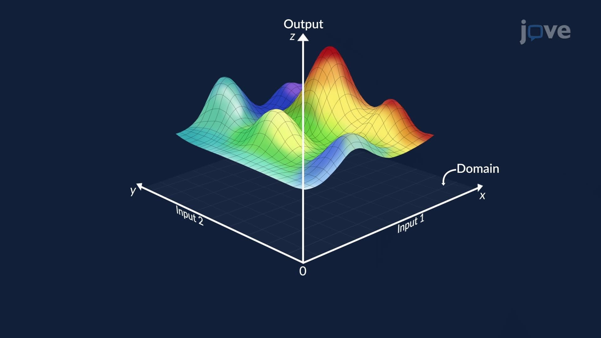
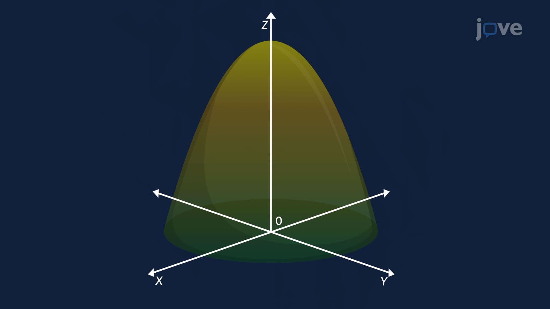
Linear approximations extend a powerful single-variable calculus idea into higher dimensions. In single-variable calculus, the tangent line at a point on a curve gives a close estimate of nearby function values. In multivariable calculus, that idea scales up: the tangent plane at a point on a 3D surface serves as the local flat model. Linear approximations use this tangent plane to estimate the value of a function f(x, y) at a point near a known location, without needing the full, often complex, expression for the surface.
The tangent plane is built from three pieces of information at a known point (a, b): the function value f(a, b), the partial derivative in the x-direction f_x(a, b), and the partial derivative in the y-direction f_y(a, b). The linear approximation formula reads:
L(x, y) = f(a, b) + f_x(a, b) · (x − a) + f_y(a, b) · (y − b)
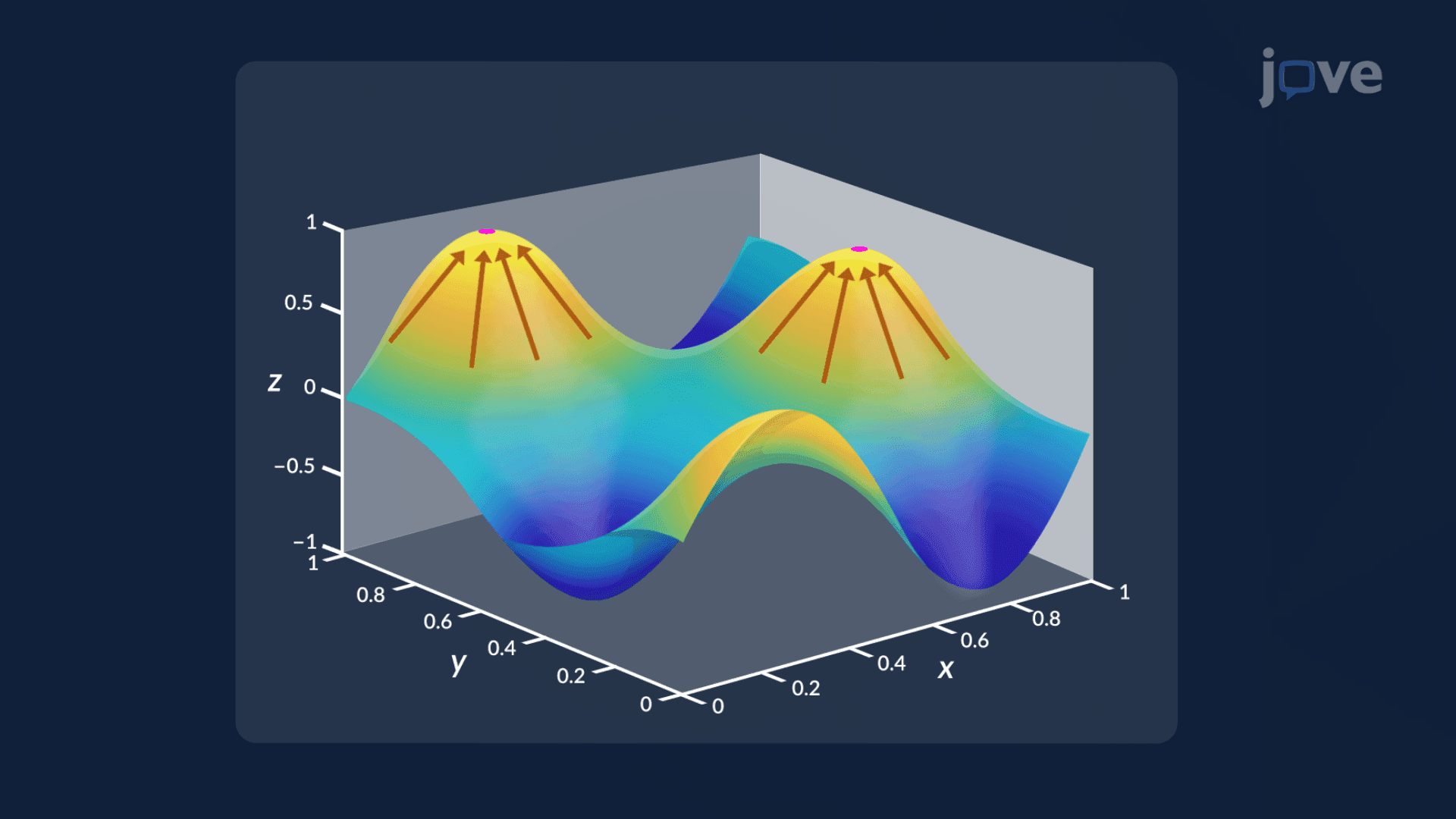
Each partial derivative captures how steeply the surface rises or falls in one direction. Together, they define the orientation of the flat plane that "kisses" the surface at (a, b). This is directly connected to the gradient of a function, the vector [f_x, f_y], which points in the direction of steepest ascent and determines the slope of the tangent plane in any direction.
Linear approximations are not just textbook exercises, they appear in active US scientific and engineering practice. The National Oceanic and Atmospheric Administration (NOAA) uses differentiable models to interpolate temperature or pressure readings between weather stations. Civil engineers estimating structural stress at points between sensor locations rely on local linear models. In medical imaging, gradient-based approximations help reconstruct tissue density from MRI scan data. Any time a complex surface must be evaluated quickly and exactly at a specific point is computationally expensive, a linear approximation offers a practical shortcut.
In AP Calculus BC, linear approximation appears as tangent line approximation for single-variable functions, a direct conceptual predecessor. College students in Calculus III (Multivariable Calculus) encounter the full tangent plane version on midterms and finals, often paired with topics like directional derivatives, higher-order partial derivatives, and maximum and minimum values of functions of two variables. Understanding linear approximations also underpins the chain rule for partial derivatives and helps interpret the geometric meaning of the gradient vector. On college exams, a typical question asks students to write L(x, y) at a given point and use it to estimate a nearby value, so being fluent in the formula and its components is essential for strong performance.
A critical insight is that linear approximations are local tools. They work best when the evaluation point (x, y) is very close to the base point (a, b). As the distance grows, the actual curved surface pulls away from the flat tangent plane, and the estimate becomes less reliable. This is why higher-order approximations, such as quadratic or Taylor series expansions, exist for cases where a wider range of accuracy is needed. Recognizing this limitation is itself a tested skill in multivariable calculus courses and reinforces why understanding the curvature of a surface matters when pushing beyond linear methods.
Related Micro-courses