Loading video…


 24 Concepts
 92 views

Video Summary: One Constraint in Lagrange Multipliers
How do engineers design the most efficient fencing layout without wasting a single meter? One constraint in Lagrange multipliers solves exactly this kind of problem. In a classic US calculus example, a rectangular pen built against a barn wall uses exactly 100 meters of fencing across three sides, and Lagrange multipliers find the dimensions that maximize the enclosed area. Watch the full video on JoVE Coach to master this concept with expert-led visuals and step-by-step explanations.
Constrained optimization is everywhere, from a national park designing wildlife enclosures to a startup minimizing production costs with a fixed budget. One constraint in Lagrange multipliers is the foundational technique that handles these situations mathematically. Introduced in college-level multivariable calculus courses across the US, including AP Calculus BC extensions and standard Calculus III curricula, this method elegantly fuses geometry, algebra, and the power of partial derivatives into a single structured approach.
Every Lagrange multiplier problem has two essential ingredients. The first is the objective function, the quantity you want to maximize or minimize. In the classic fencing example, this is the area A = L × W, where L is the length of the pen and W is the width. The second is the constraint equation, the condition that limits your choices. Here, because the barn wall forms one side, only three sides need fencing, giving the constraint L + 2W = 100.
Setting up these two expressions correctly is the most critical step. Students who struggle with Lagrange multiplier problems almost always trace the difficulty back to misidentifying which function is the objective and which is the constraint, not to the calculus itself.
Here is where multivariable calculus becomes visually powerful. In the length-width plane, the constraint L + 2W = 100 is a straight line, a curve that limits all possible pen dimensions. The objective function A = L × W produces a family of level curves, each representing a constant area. As you increase the target area, these hyperbolic level curves shift outward. The maximum feasible area occurs at the exact point where a level curve just barely touches the constraint line, they share a common tangent at that point.
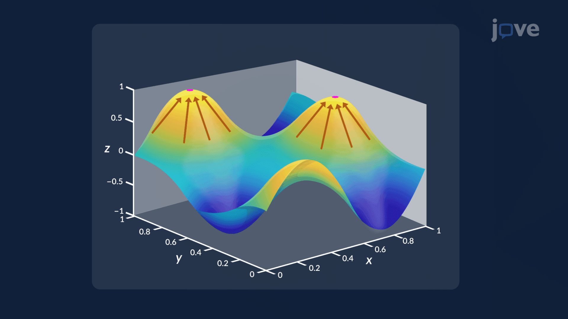
The geometric interpretation of the gradient vector makes this precise: at that point of tangency, the gradient of the area function and the gradient of the constraint function must point in the same direction, they are parallel. Because parallel vectors can differ in scale, one is a scalar multiple of the other. That scalar is lambda (λ), the Lagrange multiplier. This gives the core condition: grad(A) = λ · grad(g), where g(L, W) = L + 2W − 100 = 0.
Taking partial derivatives with respect to L and W turns the geometric condition into an algebraic system. The partial derivative of A with respect to L equals W, and with respect to W equals L. The partial derivatives of the constraint g are both constants. Setting up the Lagrange equations gives W = λ and L = 2λ, which directly implies L = 2W. This relationship, optimal length is twice the optimal width, is substituted back into the constraint equation. Solving gives W = 25 meters and L = 50 meters, producing a maximum area of 1,250 square meters.
This structured substitution process mirrors skills tested in college midterms and Calculus III exams nationwide. Understanding how to move fluently between the gradient condition, the system of equations, and the constraint substitution is essential for exam success.
Lagrange multipliers with one constraint appear in economics (maximizing utility subject to a budget), engineering (optimizing structural dimensions under material limits), and data science (regularized regression models). In US university courses, this topic typically appears midway through Calculus III, after students have built fluency with chain rule for partial derivatives, directional derivatives, and maximum and minimum values of functions of two variables. Mastering it here unlocks more advanced topics like multiple constraints, inequality constraints, and the foundations of mathematical optimization used in machine learning.
Related Micro-courses