Loading video…

 17 Concepts
 107 views

Video Summary: What are Double Integrals
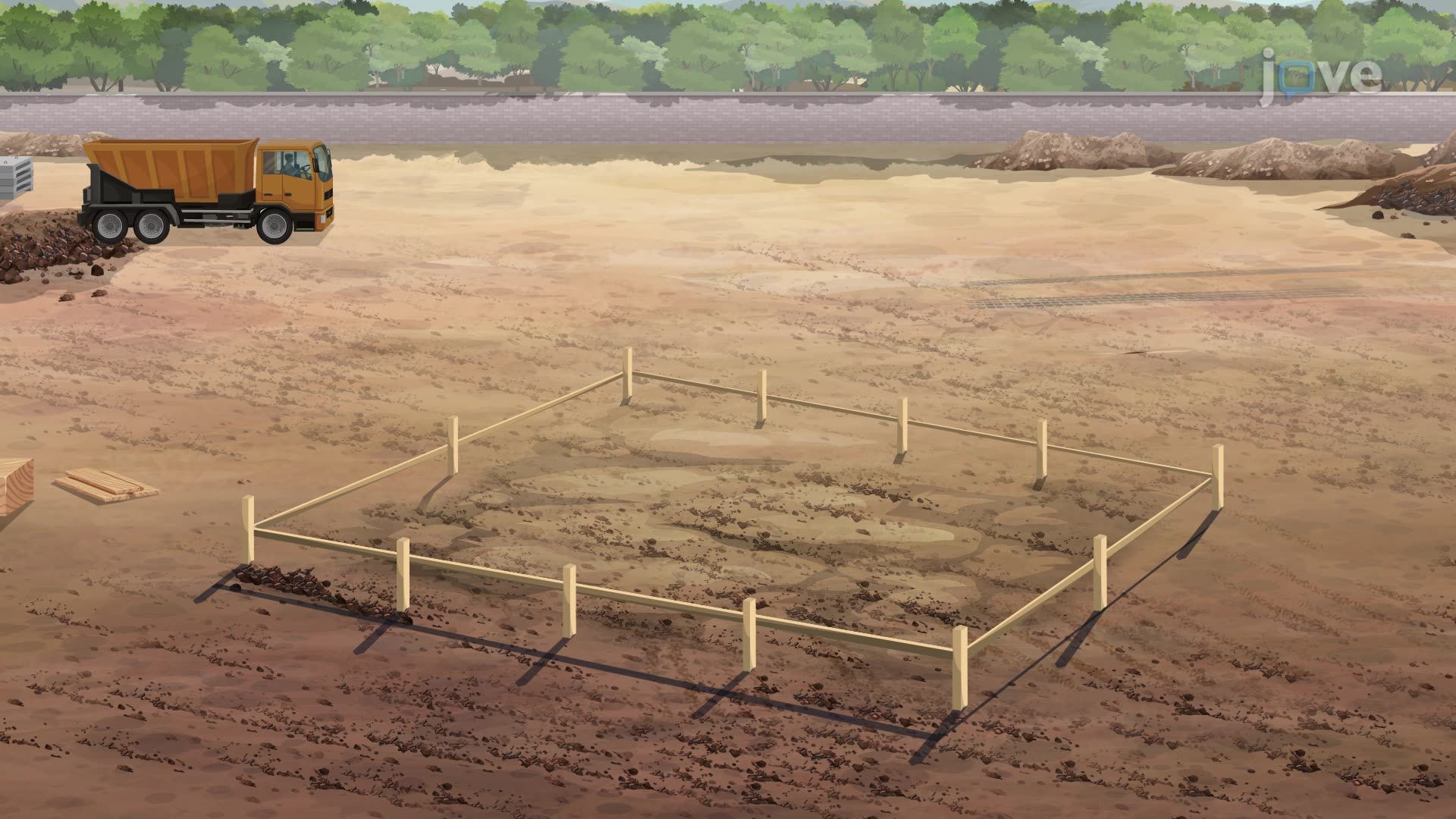
How do engineers calculate the exact amount of soil removed during a highway excavation project in Texas? Double integrals make that possible. Double integrals basics involve summing infinitely many infinitely thin volume slices beneath a 3D surface over a 2D region. By refining a grid of rectangles to the limit, the double integral captures exact volume. Watch the full video on JoVE Coach to master this concept with expert-led visuals and step-by-step explanations.
A single integral measures area under a curve. Double integrals take that logic one dimension further, they measure volume beneath a surface defined by a function of two variables, f(x, y), over a region in the xy-plane. This is a cornerstone concept in multivariable calculus, typically encountered in Calculus III at US colleges or in AP Calculus BC extensions and university STEM programs.
The foundation of double integrals is the double Riemann sum. Imagine dividing a rectangular region on the xy-plane into a grid of small rectangles, each with area ΔA = Δx · Δy. For each small rectangle, you pick a sample point (x*, y*) and evaluate the function f(x*, y*), this gives the height of the surface at that point. Multiplying height by area gives the volume of a thin rectangular column. Summing all such columns across the entire grid approximates the total volume beneath the surface.
As the grid becomes finer, meaning the number of rectangles increases and each ΔA shrinks toward zero, this approximation converges to an exact value. That limit is formally defined as the double integral of f over the region R, written as the double integral of f(x, y) dA over R. This process directly mirrors how single-variable integrals are derived, making it an intuitive generalization.
In practice, double integrals are evaluated using iterated integrals, integrating one variable at a time while treating the other as a constant. For a rectangular region where x runs from a to b and y runs from c to d, the double integral equals the integral from a to b of [the integral from c to d of f(x, y) dy] dx. This is called Fubini's Theorem, and it transforms a 2D problem into two sequential 1D integrations.
For example, a civil engineering student at UCLA calculating material volume for a curved retaining wall would set up exactly this kind of iterated integral, assigning x and y bounds to match the physical dimensions of the wall's footprint.
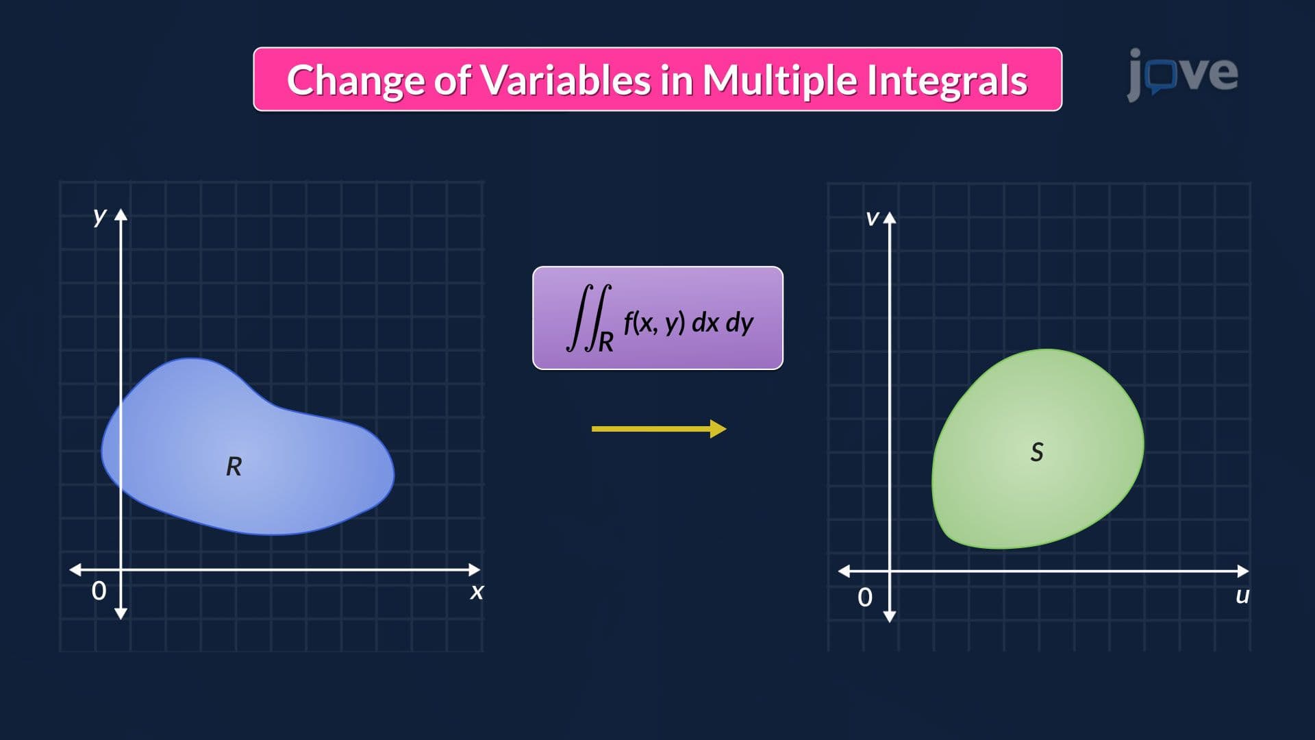
Not every real-world region is a neat rectangle. When the boundary of a region curves, like the base of a circular water reservoir in Arizona, polar coordinates integration becomes far more efficient. By substituting x = r cos(θ) and y = r sin(θ), and replacing dA with r dr dθ, the double integral adapts cleanly to circular and radial domains. The factor r in r dr dθ is a simple case of the Jacobian, which accounts for how area elements stretch or compress during coordinate transformations.
Double integrals also scale directly into triple integrals for three-dimensional solids, and they power applications like center of mass using multiple integrals, probability density functions in statistics, and heat distribution modeling in physics. On college midterms and finals in Calculus III, students are routinely asked to set up and evaluate double integrals over both rectangular and general regions, making fluency with this concept essential for success in STEM coursework.
Related Micro-courses