Multiple Integrals and Applications

Multiple Integrals and Applications Principles form the backbone of Calculus 3, extending single-variable integration into two and three dimensions. From calculating excavation volumes on US construction sites to modeling snowfall across Colorado, this micro-course — supported by JoVE Coach — covers double and triple integrals, polar, cylindrical, and spherical coordinates, Jacobians, and real-world applications including center of mass and surface area.

• Understand how double and triple integrals generalize the concept of accumulation across two- and three-dimensional regions
• Learn to evaluate iterated integrals using Fubini's Theorem and apply it to problems involving variable density and mass
• Identify Type I and Type II regions and set up double integrals over general, non-rectangular domains with variable bounds
• Explore polar, cylindrical, and spherical coordinate systems and recognize when each simplifies multiple integrals calculus 3 problems
• Apply surface area formulas and triple integrals to solve engineering and physics problems, such as satellite dish fabrication and storage tank volumes
• Analyze how changing the order of integration in double and triple integrals can reduce computational complexity
• Apply the Jacobian to perform change-of-variables transformations that convert complex regions into simpler integration domains
• Calculate moments and centers of mass for laminar plates with variable density using double integrals

1. Introduction to Double Integrals and the Midpoint Rule A double integral measures the exact volume beneath a surface defined over a two-dimensional region. The concept begins with a double Riemann sum, where a region is divided into small subrectangles, a height value is sampled at each, and the resulting rectangular columns are summed. As the subrectangles shrink in size, the Riemann sum converges to the exact double integral. The Midpoint Rule offers a practical approximation technique by sampling each subrectangle at its center point. In US civil engineering projects, for example, this method estimates earthwork volumes by evaluating terrain elevation at midpoints across a gridded rectangular region, making it a useful field-level computational tool before exact integrals are solved.

2. Iterated Integrals and Fubini's Theorem Evaluating a double integral directly is rarely practical, so it is rewritten as an iterated integral — two nested single integrals computed sequentially. The inner integral is solved first by holding one variable constant, and the result is then integrated with respect to the remaining variable. Fubini's Theorem guarantees that for a continuous function over a rectangular region, both possible orders of integration — integrating with respect to x first or y first — produce identical results. This flexibility is invaluable in applications such as computing the total mass of a thin plate with variable material density, where one integration order may produce far simpler algebra than the other.

3. Average Value of a Function Over a Region The average value of a multivariable function over a two-dimensional region is computed by dividing the double integral of the function by the total area of the region. This directly extends the single-variable average value formula into two dimensions. A practical US example involves mapping average snowfall depth across a rectangular portion of Colorado over a given time period. Using the Midpoint Rule to approximate the double integral, the region is subdivided, snowfall values are sampled at midpoints, area-weighted contributions are summed, and dividing by the total area yields the spatial average — a method used widely in meteorology and environmental science.

4. Double Integrals Over General Regions and Changing Order of Integration Not all real-world domains are rectangular. Double integrals over general regions are handled by classifying the domain as either Type I, bounded by two functions of x between constant vertical limits, or Type II, bounded by two functions of y between constant horizontal limits. Variable bounds replace constant limits in the iterated integral setup. When the original integration order leads to difficult or unsolvable integrals — for example, when boundary curves are complex — reversing the order of integration often resolves the problem. Although the mathematical region remains unchanged, re-describing it along a different axis can dramatically simplify the limits and the resulting computation.

5. Double Integrals in Polar Coordinates Polar coordinates express a point in the plane using a radial distance r from the origin and an angle θ, making them the natural choice for circular or symmetric regions. Converting a double integral to polar form replaces x and y with r·cos θ and r·sin θ, and the area element dA becomes r·dr·dθ — the extra factor r accounts for the increasing arc length of sectors farther from the origin. This transformation eliminates the square-root expressions that arise in Cartesian limits for circular boundaries. A landscape architecture example — finding the concrete area of a semicircular pond — illustrates how polar coordinates reduce a complicated Cartesian integral into a clean, straightforward computation.

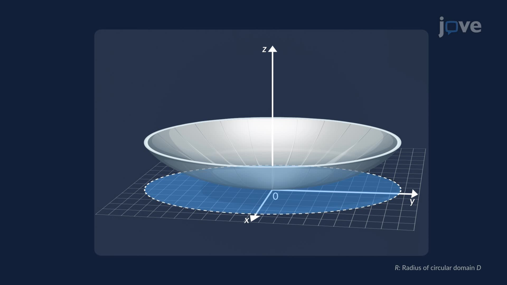
6. Surface Area Calculations Using Double Integrals The surface area of a curved three-dimensional surface defined as z = f(x, y) is calculated using a double integral that incorporates the partial derivatives of f. The integrand includes the square root of the sum of the squares of ∂z/∂x and ∂z/∂y, plus one — a term that captures the local steepness of the surface. For a parabolic satellite dish with a circular base region, polar coordinates simplify the integral domain. This approach gives engineers the exact reflective surface area needed to estimate the amount of protective coating required and to calculate precise material costs during the fabrication process.

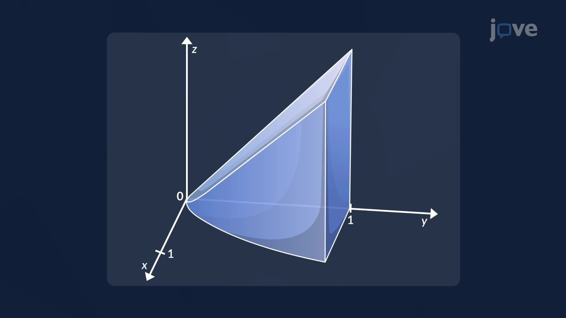
7. Triple Integrals in Rectangular Coordinates and Over General Regions Triple integrals extend accumulation into three-dimensional space. A solid region is subdivided into tiny sub-boxes, a function value (such as density) is sampled in each, multiplied by the sub-box volume, and the limit of this sum defines the triple integral. Fubini's Theorem applies here too — the order of integration among x, y, and z can be changed freely for continuous functions with well-defined bounds. For a solid bounded by two surfaces, the projection of the solid onto the horizontal plane forms a base region, with vertical segments connecting the lower and upper boundary surfaces. This framework applies directly to estimating the volume or mass of irregularly shaped geological ore deposits.

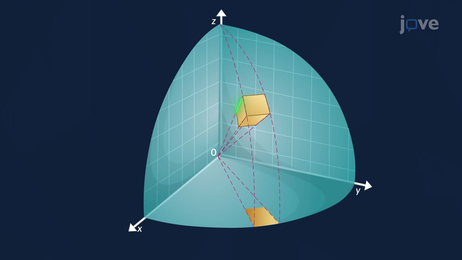
8. Triple Integrals in Cylindrical and Spherical Coordinates Cylindrical coordinates (r, θ, z) augment polar coordinates with a vertical component and are best suited for regions with circular cross-sections, such as storage tanks or cylindrical machine parts. The volume element becomes r·dr·dθ·dz. Spherical coordinates (ρ, θ, φ) describe points by distance from the origin, azimuthal angle, and polar angle, and the volume element is ρ²·sin φ·dρ·dθ·dφ. These coordinate systems are ideal for deriving standard formulas — the volume of a cylinder or sphere — and for solving problems in physics and engineering where the geometry has natural rotational symmetry, such as modeling a paraboloid-shaped water tank or calculating gravitational fields.

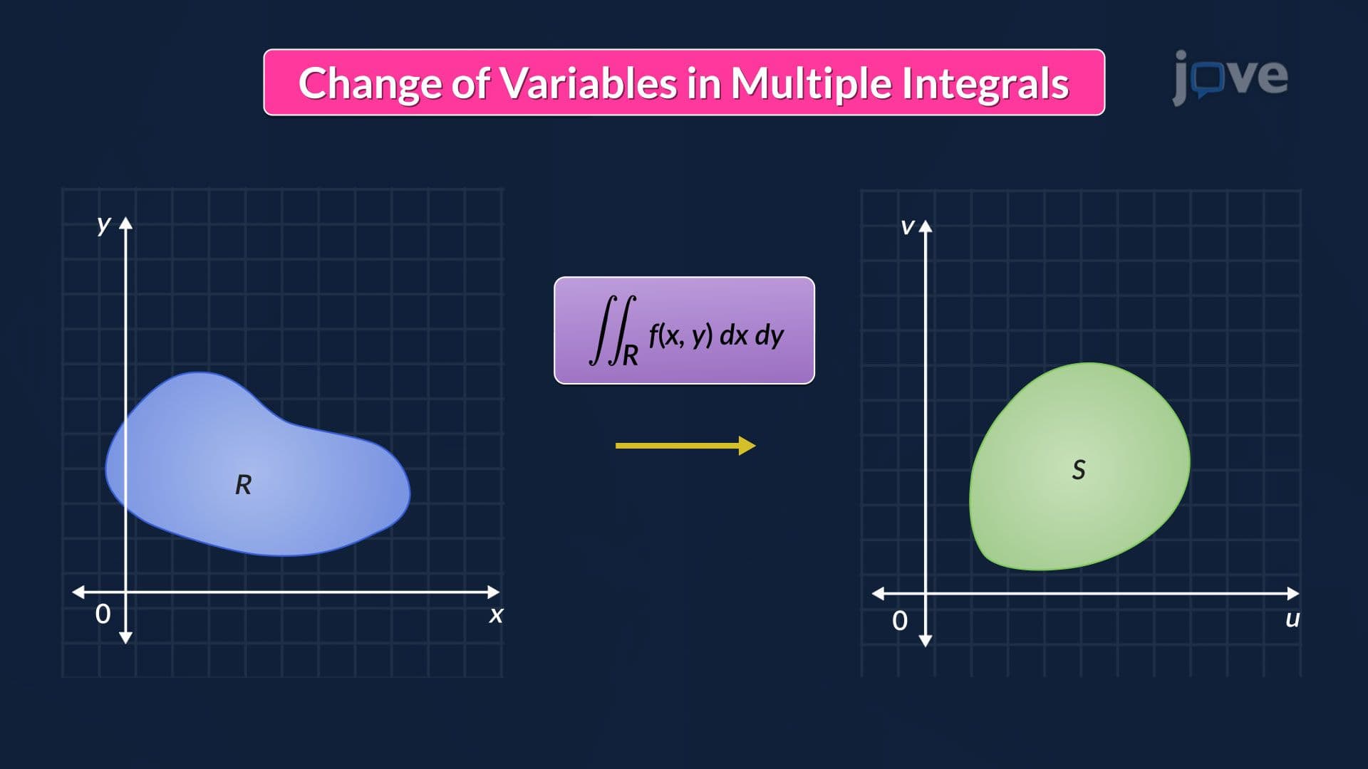
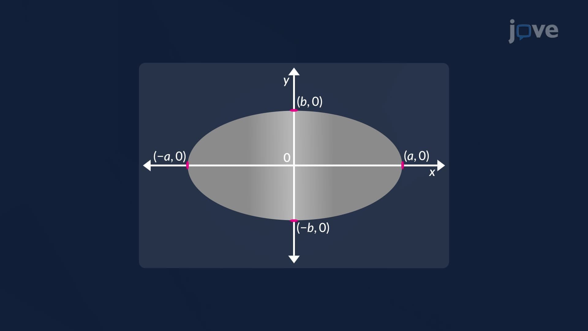
9. Change of Variables and the Jacobian in Multiple Integrals When a region of integration has an inconvenient shape in standard coordinates, a change of variables transforms it into a simpler domain. The Jacobian is the determinant of the matrix of partial derivatives of the original variables with respect to the new variables, and its absolute value corrects for how the transformation stretches or compresses area or volume. For an elliptical metal plate, substituting x = au and y = bv maps the ellipse to a unit circle, simplifying the boundary conditions entirely. A second transformation to polar coordinates then reduces the integral to one with constant limits. Each transformation introduces its own Jacobian factor, and both must be included in the final integral.

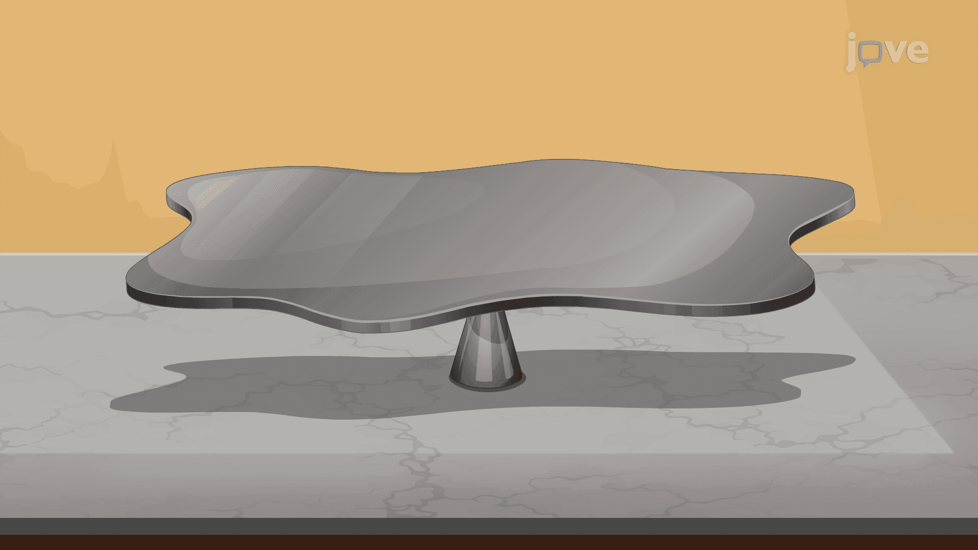
10. Moments, Centers of Mass, and Real-Life Applications The center of mass of a flat plate with variable density is found using double integrals to compute total mass and the moments about each axis. The moment about the x-axis weights mass elements by their vertical distance, while the moment about the y-axis weights them by horizontal distance. Dividing each moment by the total mass gives the coordinates of the center of mass. This principle applies in aerospace engineering, structural design, and robotics. More broadly, multiple integrals are used across US industries — from estimating reservoir water volumes in civil engineering to modeling probability distributions in statistics and computing charge distributions in electromagnetic systems.