Applications of Integration

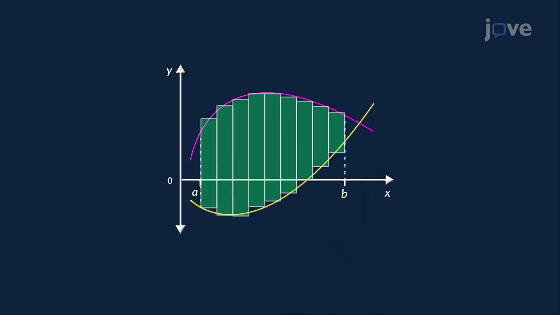
Integration Applications explores how definite integrals solve real-world measurement problems across engineering, economics, and science. From calculating the area between curves to finding volumes of complex solids and average function values, this micro-course — supported by JoVE Coach — connects core calculus concepts to authentic US applications, including income inequality analysis, jet fuel tank design, and greenhouse temperature monitoring.

• Understand how to set up and evaluate definite integrals to find the area between two curves with respect to both x and y
• Learn how to apply the Slicing Method to compute volumes of irregular solids by integrating cross-sectional areas
• Identify when to use the Disk Method for solids of revolution and how axis orientation affects the integral setup
• Explore how cross-sectional geometry — including equilateral triangles — determines volume in non-standard three-dimensional shapes
• Analyze multi-segment regions by splitting integration intervals at points of intersection between boundary curves
• Apply the average value formula to interpret a definite integral as the mean output of a continuous function over a closed interval
• Connect integration techniques to real-life contexts such as consumer surplus in economics and fuel tank volume in aerospace engineering

1. Area Between Curves — Integrating with Respect to x When two continuous functions are defined over a closed interval [a, b], the area of the region between them is found by integrating the vertical distance between the upper and lower curves with respect to x. This is derived from the Riemann sum approach: the region is divided into thin vertical rectangles, and as their width shrinks toward zero, the sum converges to a definite integral. In US economics courses, this technique directly models the Gini coefficient — the area between the line of perfect income equality and the actual Lorenz curve — used by the Census Bureau to measure income inequality across American households.

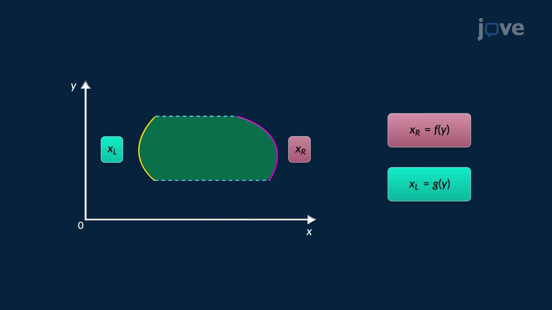
2. Area Between Curves — Integrating with Respect to y Some regions are more naturally described by functions of y, where boundaries run left and right rather than up and down. In this case, horizontal strips of width Δy replace vertical ones, and integration is performed along the y-axis from y = c to y = d. The integrand becomes the horizontal distance between the right and left boundary curves. This approach is essential when a single function of x fails to describe the entire boundary without splitting the integral. In chemical engineering, this method appears in vapor-liquid equilibrium diagrams, where the enclosed area between the equilibrium curve and the diagonal measures the theoretical separation potential of a mixture component.

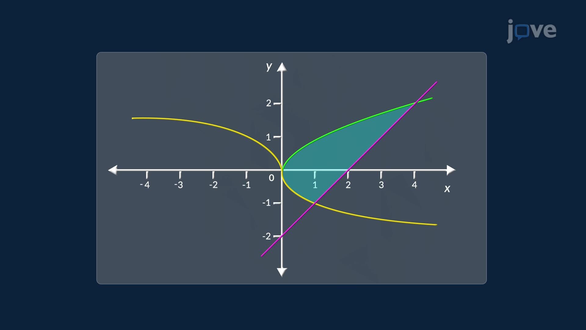
3. Area Between Curves — Multi-Region Problem Solving When boundary curves intersect at interior points, the region must be divided into segments, each with its own pair of upper and lower boundaries. A definite integral is written for each sub-interval, and the total area is the sum of all segment integrals. Identifying the correct upper and lower functions in each interval is critical — swapping them produces a negative value. This technique is applied in welfare economics to calculate total economic surplus. The demand and supply curves intersect at the equilibrium price; integrating the vertical gap from zero to equilibrium quantity captures both consumer and producer surplus — a measure central to US microeconomics and public policy analysis.

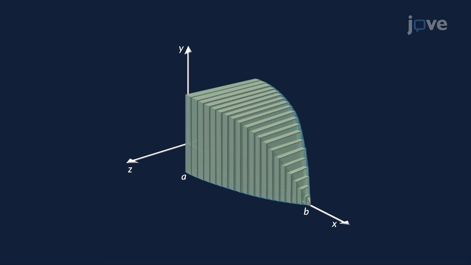
4. Volume by Slicing — The Slicing Method For solids with variable cross-sections, volume cannot be computed with a simple formula. The Slicing Method treats the solid as a stack of infinitely thin slices perpendicular to a chosen axis. Each slice has cross-sectional area A(x) and thickness dx, contributing a volume element of A(x) dx. A definite integral over the length of the solid sums all these contributions exactly. Civil engineers in the US use this method to estimate the volume of concrete in arch dams or irregularly shaped retaining structures, where cross-sections vary along the length and material cost estimates depend on precise volume calculations.

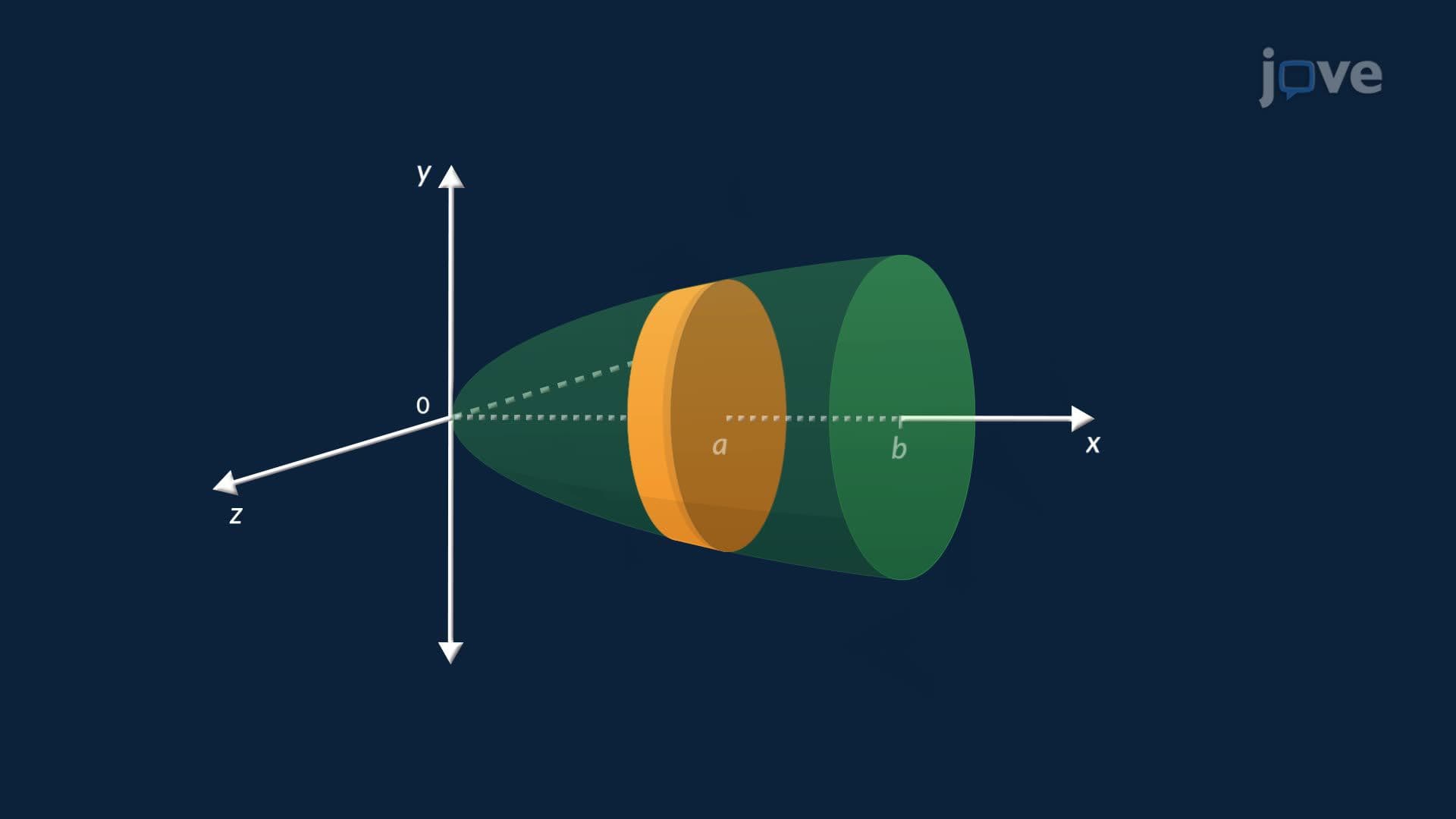
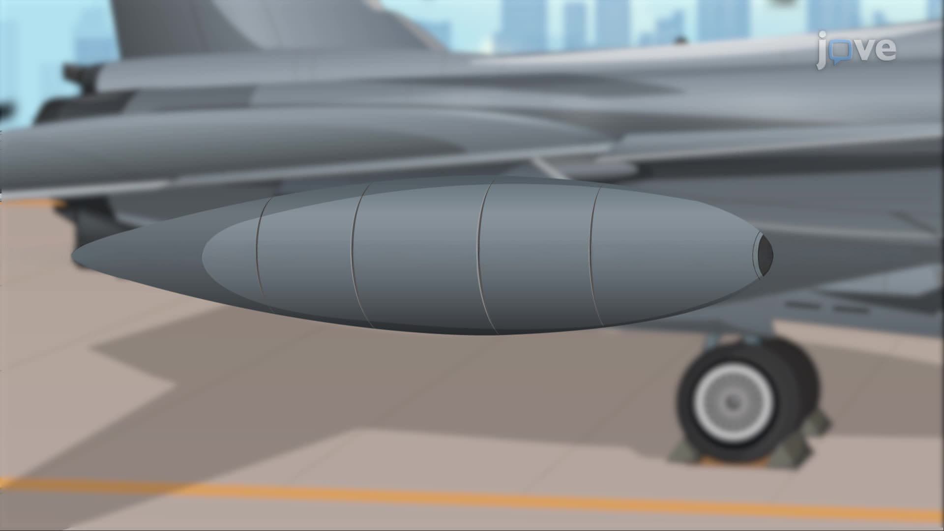
5. Volumes of Solids of Revolution — The Disk Method When a two-dimensional region is rotated around an axis, it sweeps out a three-dimensional solid of revolution. If the region sits directly against the axis, every cross-section perpendicular to that axis is a solid circle — a disk. The Disk Method integrates the area of these circular cross-sections, where the radius of each disk equals the function's value at that x-position. The volume of each disk is π[r(x)]² dx, and integrating over the interval gives the total volume. This method is used in aerospace engineering to calculate the internal volume of wing-mounted fuel tanks shaped by rotating a mathematical profile curve, ensuring accurate fuel capacity specifications for aircraft design.

6. Volume Using Cross-Sectional Area — Non-Circular Shapes Not all cross-sections are circular. When cross-sections have a defined geometric shape — squares, rectangles, triangles, or semicircles — their areas can be expressed as functions of position along the axis, then integrated to find total volume. For example, a tetrahedron with equilateral triangular cross-sections has cross-sectional area proportional to y², and integrating from apex to base recovers the standard volume formula. In practice, land surveyors and civil engineers measure cross-sections of irregular gravel stockpiles or earthwork fills at regular intervals along a site, then integrate those measurements numerically to estimate total material volume for construction projects across the US.

7. Average Value of a Function The average value of a continuous function f(x) over [a, b] is defined as the definite integral of f divided by the width of the interval (b − a). Geometrically, this equals the height of a rectangle whose area matches the net area under the curve — the Mean Value Theorem for Integrals confirms such a height always exists. This concept is used in environmental monitoring: for example, the US EPA and agricultural agencies compute average daily temperature, humidity, or pollutant concentration over a 24-hour or seasonal interval to make regulatory and operational decisions, treating continuously measured sensor data as an integrable function.