Loading video…

 8 Concepts
 3K views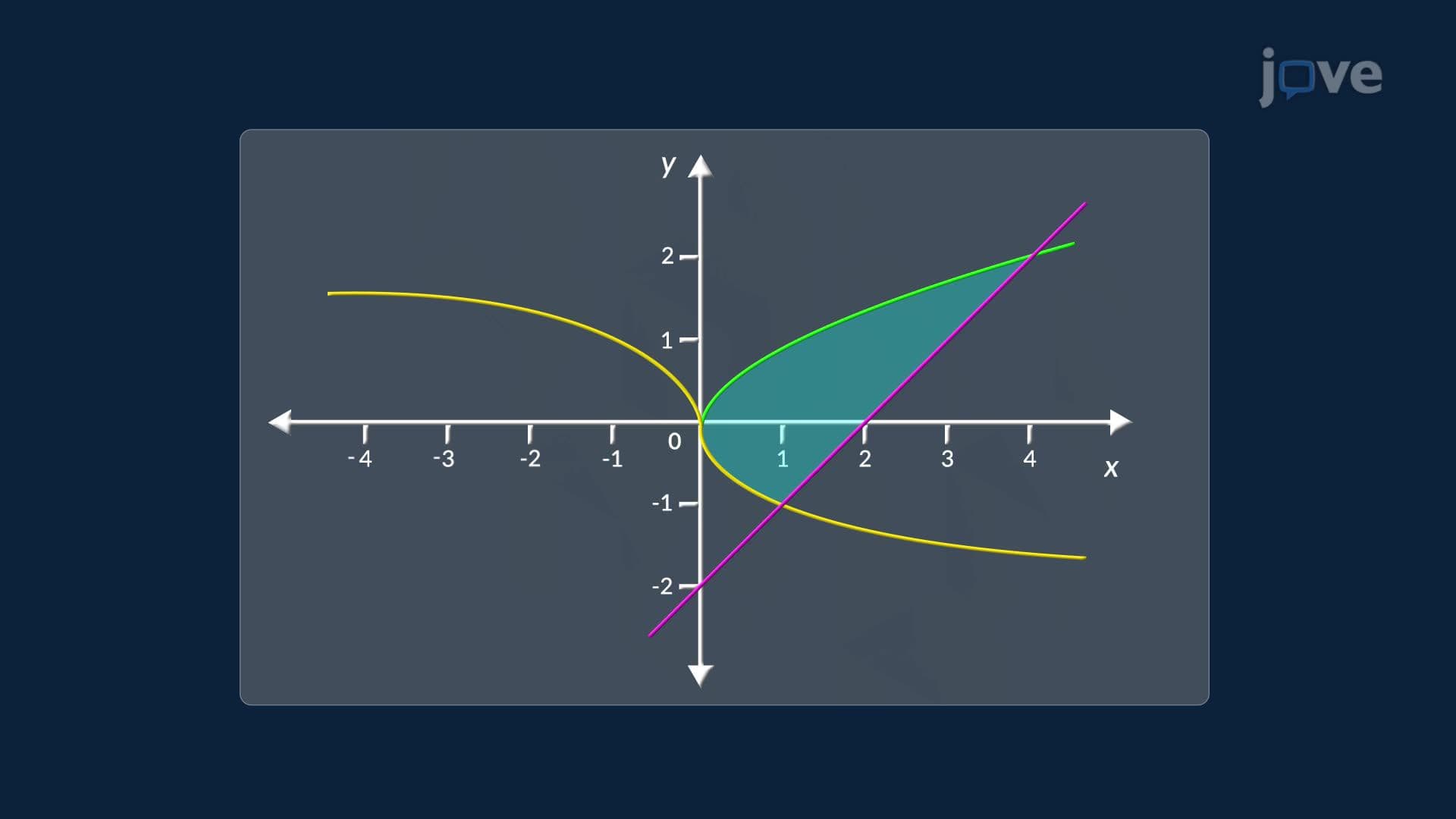

Video Summary: Problem Solving in Area Between Curves
Did you know that economists use calculus to measure billions of dollars in consumer and producer surplus every year? Problem solving in area between curves becomes essential when boundaries shift across an interval, a challenge that appears in both math classrooms and real-world economics. In the US, welfare economists apply this exact method to analyze market efficiency using supply and demand curves. Watch the full video on JoVE Coach to master this concept with expert-led visuals and step-by-step explanations.
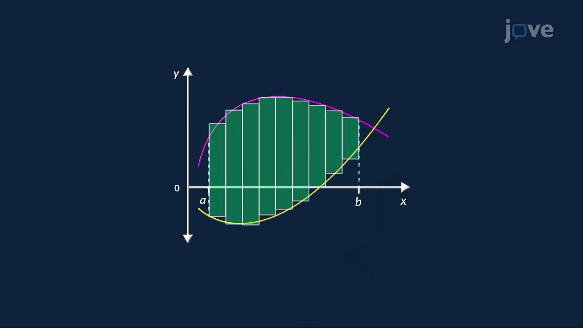
When two or more curves enclose a region that changes shape across an interval, finding the total area requires more than a single integral. Problem solving in area between curves is the structured process of identifying boundaries, locating intersection points, splitting the region into manageable segments, and integrating across each one. This skill is central to Calculus AB and BC courses, frequently tested on the AP Calculus exam, and revisited in college-level Calculus II courses across the US.
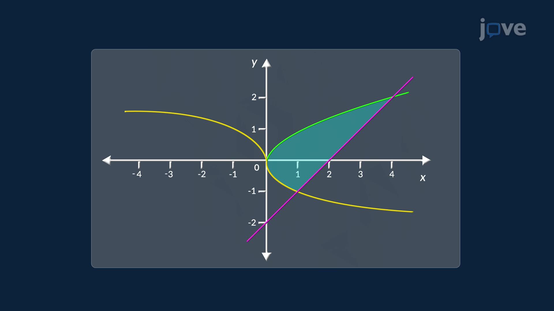
The first step is always to determine which curve sits on top and which sits on the bottom throughout the region. When curves include functions like f(x) = sqrt(x), g(x) = -cbrt(x), and a linear function, the relative positions can shift at intersection points. Setting functions equal to each other reveals these crossover points. For a region bounded between x = 0 and x = 4 with an intersection at x = 1, the region naturally divides into two sub-intervals: [0, 1] and [1, 4]. Failing to split at these crossover points is one of the most common errors students make on AP Calculus free-response questions.
Once the boundaries are confirmed for each sub-interval, the area formula becomes straightforward. For each segment, the area equals the definite integral of [upper curve minus lower curve] with respect to x, evaluated over that interval. The total area is the sum of both definite integrals. In plain text:
Total Area = integral from 0 to 1 of [f(x) - g(x)] dx + integral from 1 to 4 of [h(x) - k(x)] dx
Careful evaluation of each integral, including proper handling of fractional exponents, is essential. Students preparing for AP Calculus exams should practice both the setup and the arithmetic, since partial credit depends on correctly identifying boundaries even when the final numerical answer contains errors.
One of the most compelling US applications of this method appears in welfare economics. Economists at institutions like the Congressional Budget Office or in undergraduate economics courses at universities like Harvard and UC Berkeley use area-between-curves calculations to measure consumer surplus, producer surplus, and total economic surplus. The demand curve forms the upper boundary, the supply curve forms the lower boundary, and the equilibrium quantity defines the right endpoint of integration. The area of that enclosed region, calculated by integrating the vertical difference between the two curves from zero to equilibrium, represents the net economic benefit generated by a market. This makes the integral not just an abstract calculation, but a tool with measurable policy implications.
Mastering this technique unlocks a broader toolkit. The same logic of integrating a difference between two boundaries extends to volume by slicing, where cross-sectional areas replace curve differences. It also connects to finding the center of mass of a laminar region, computing arc length along a curve, and determining the surface area of revolution. Understanding what integration is used for, beyond pure mathematics, helps students see these techniques as interconnected rather than isolated procedures. Each concept builds directly on the ability to set up and evaluate a definite integral over a carefully defined interval.
Related Micro-courses