Area Between Curves: Integrating With Respect to x

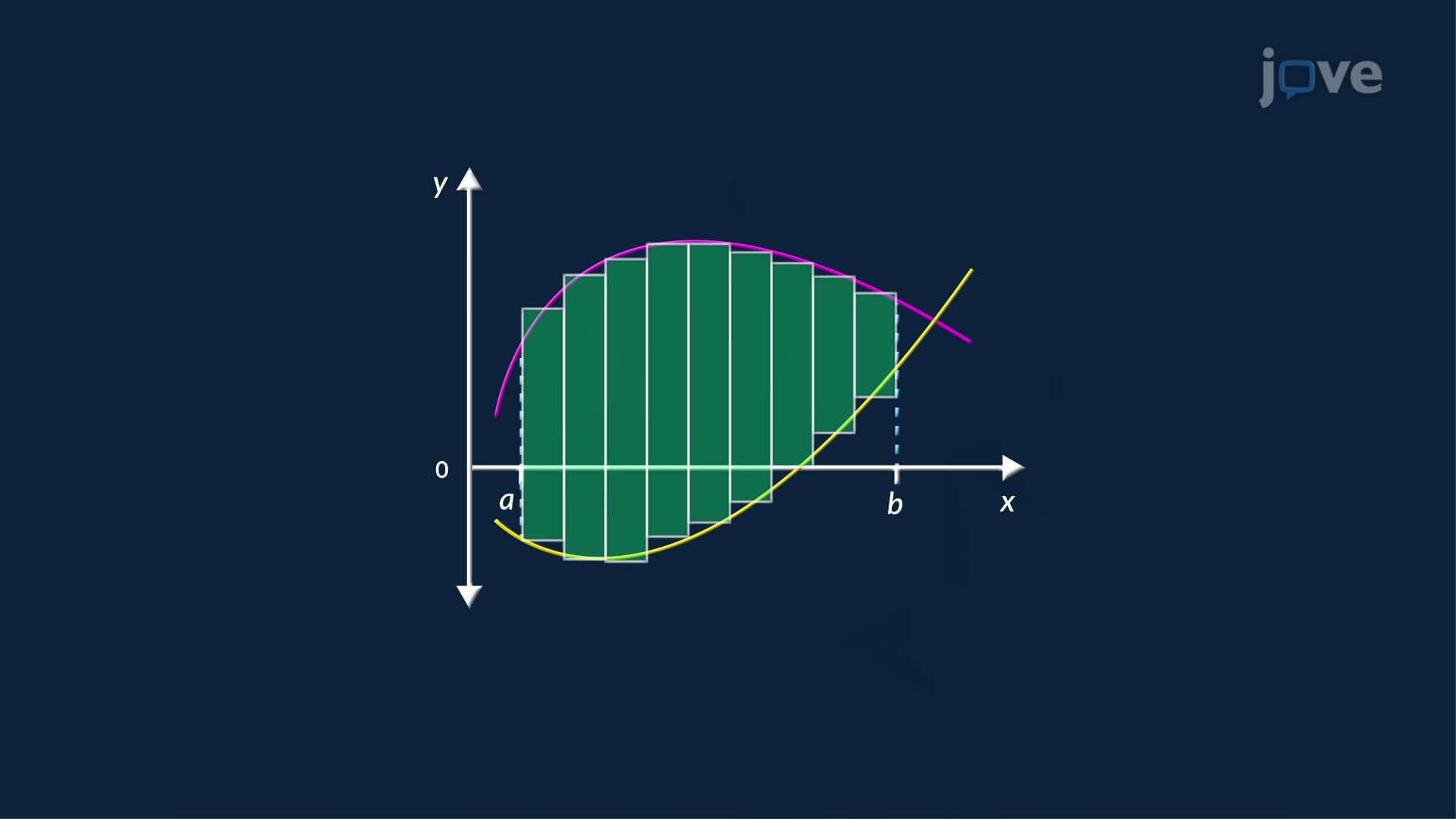
• Understand how *Integrating with Respect to X in Area Between Curves* builds on the Riemann sum approach to produce an exact area calculation using definite integrals
• Identify the upper and lower functions on a closed interval [a, b] and set up the correct integrand as f(x) minus g(x)
• Analyze how increasing the number of rectangular strips in a Riemann sum progressively approximates the true area between two curves
• Compare the limitations of finite rectangle estimation with the precision achieved through integration with infinitely thin vertical slices
• Apply the area between curves formula to solve problems involving bounded regions in AP Calculus AB and BC coursework and college-level calculus
• Recognize real-world contexts, such as income inequality analysis using the Lorenz curve, where the area between curves produces meaningful, actionable results
• Evaluate whether integrating with respect to x is the most efficient method for a given region, based on the orientation of the bounding curves
• Explore how this technique connects to broader integration applications including volume by slicing, arc length, and surface area of revolution

Integrating with Respect to X in Area Between Curves: The Core Idea

When two continuous functions share a closed interval on the x-axis, they enclose a region. Finding the exact size of that region is one of the most practical skills in calculus. *Integrating with respect to x in area between curves* solves this problem by treating the enclosed region as a collection of infinitely thin vertical slices, each with a measurable height, and summing them through integration. The result is a definite integral of the form: Area = integral from a to b of [f(x) minus g(x)] dx, where f(x) is the upper curve and g(x) is the lower curve across the entire interval.

From Rectangles to Exact Area: The Riemann Sum Connection

Before integration, the area can be estimated using the Riemann sum method. The region is divided into *n* vertical strips of equal width. Each strip is approximated as a rectangle whose height equals the vertical distance between the two curves at a chosen x-value, and whose base is the strip width. Summing the areas of all rectangles gives an estimate. The critical insight is what happens as *n* grows: as the number of rectangles approaches infinity, the estimate converges to the exact area. Integration is precisely this limiting process, it replaces the finite sum with a definite integral, eliminating the approximation error entirely.

Setting Up the Integral Correctly

Accurate setup is everything. Students must correctly identify which function is on top across the interval [a, b]. If f(x) is greater than or equal to g(x) for all x in [a, b], the integrand is simply f(x) minus g(x). If the curves cross within the interval, the region must be split at each intersection point, and separate integrals must be set up for each sub-interval. On the AP Calculus AB and BC exams, this step, correctly handling crossings, is a frequent source of lost points. Always verify by testing a value from each sub-interval to confirm which function is greater.

Real-World US Application: The Lorenz Curve and Income Inequality

One of the most compelling real-world uses of this technique appears in economics. The Lorenz curve plots the cumulative share of income earned by the bottom percentage of a population. The line of perfect equality is a straight diagonal line. The area between these two curves, calculated by integrating with respect to x, defines the inequality gap, which feeds directly into the Gini coefficient, the standard measure of income inequality used by the US Census Bureau. A larger area means greater inequality. This application demonstrates that area between curves is not an abstract exercise; it quantifies real disparities in American economic life.

Connections to Broader Calculus Topics

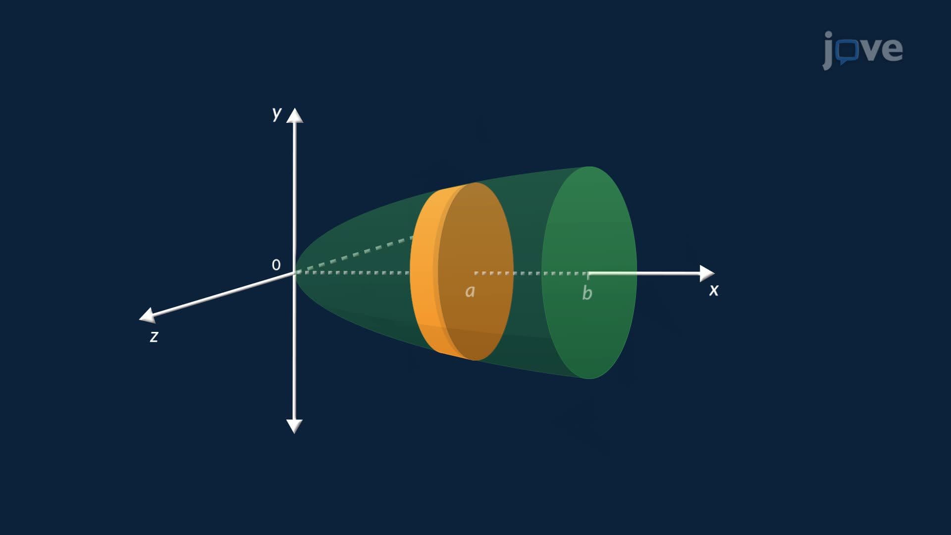
Mastering integration with respect to x in area between curves opens the door to more advanced applications. The same slicing logic underpins volume by slicing (used to find volumes of solids of revolution), arc length, surface area of revolution, and center of mass calculations. These topics appear in college-level Calculus II courses at universities across the US, including in engineering, physics, and economics programs. Students who solidify this foundational concept find the transition to those topics significantly smoother.