Partial Derivatives and Gradients

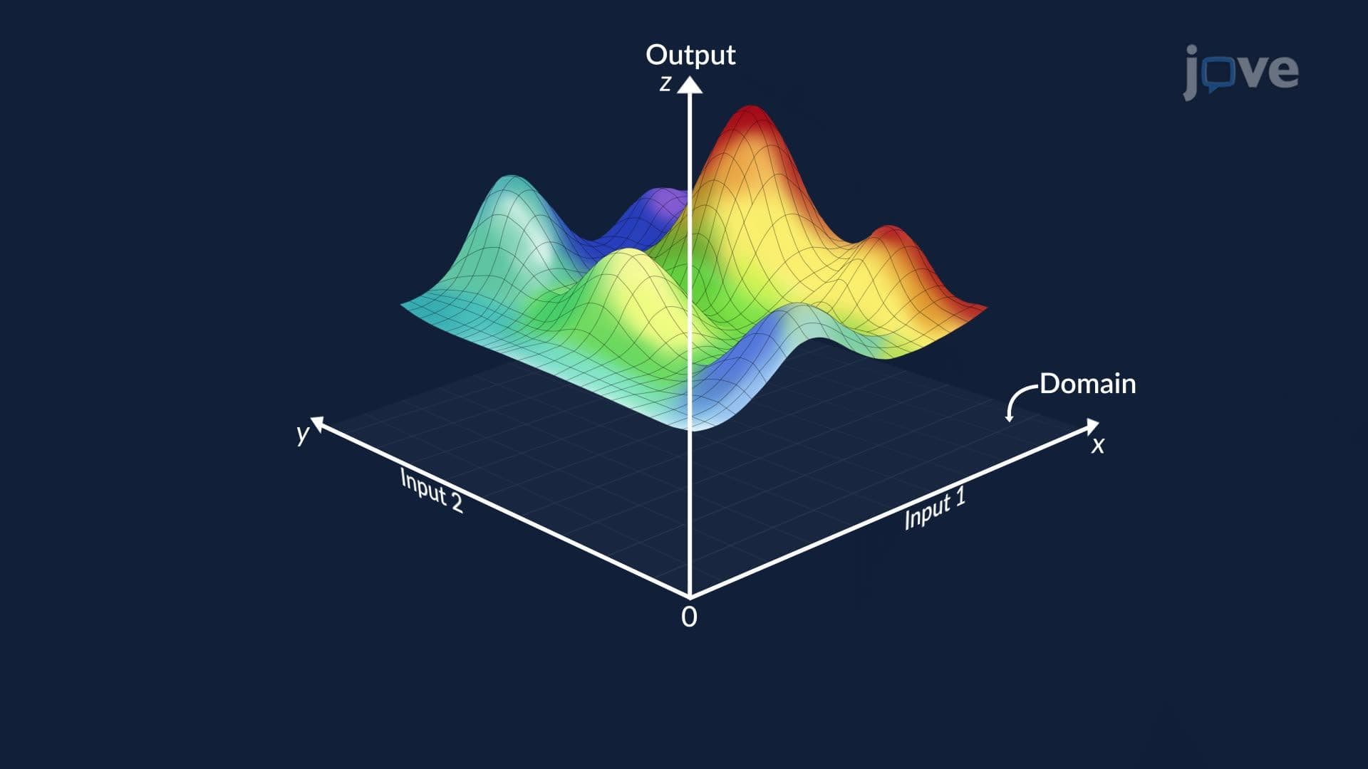
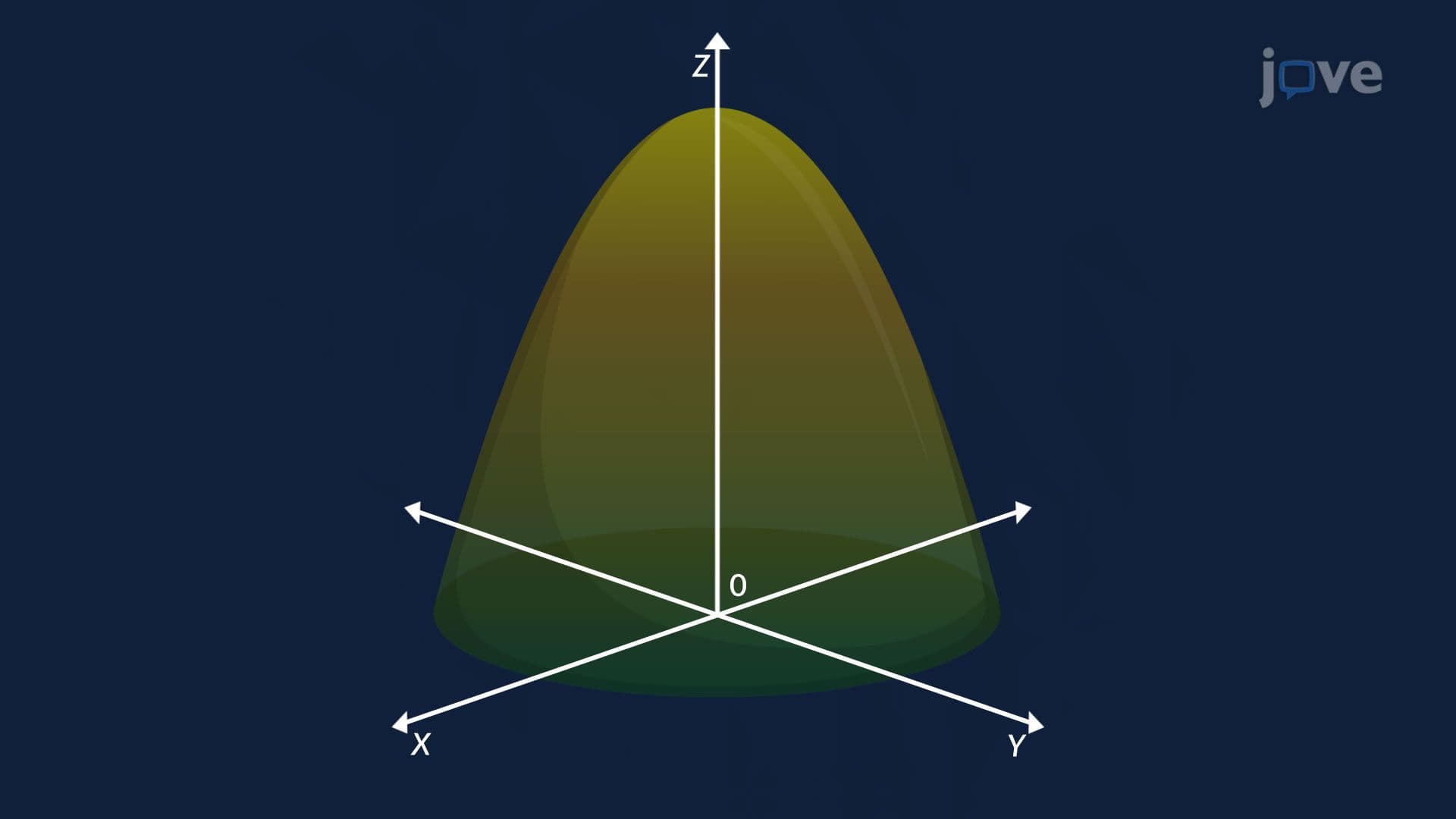
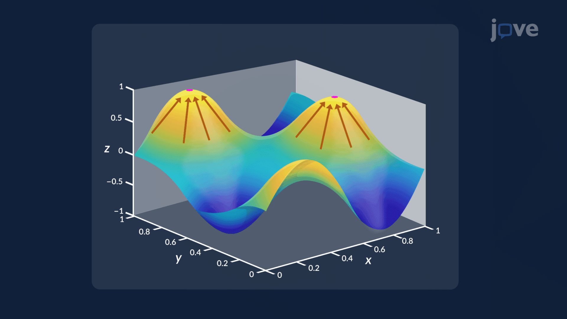
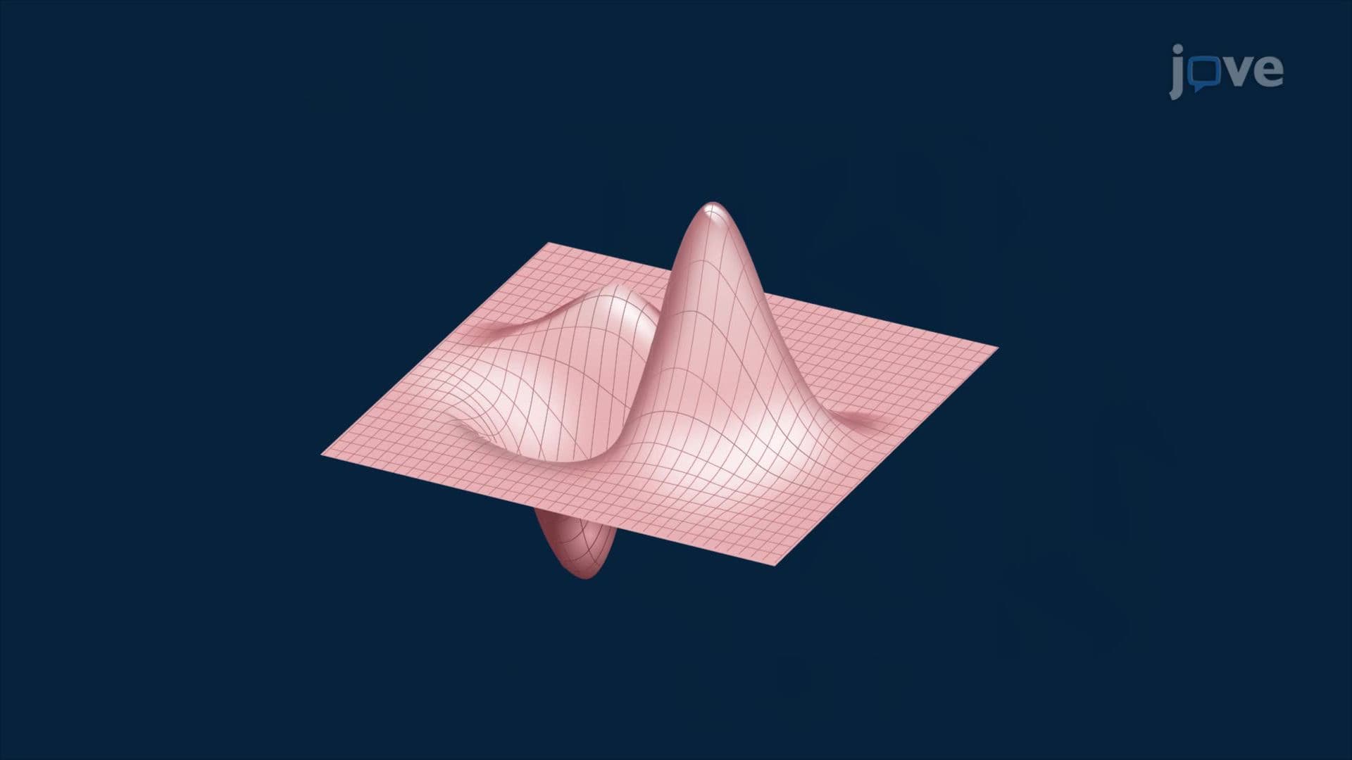
Partial derivatives and gradient vector calculus form the mathematical backbone of modern science and engineering. This micro-course, powered by JoVE Coach, builds from functions of two variables through contour maps, limits, continuity, tangent planes, directional derivatives, and Lagrange multipliers. US-relevant applications — from weather modeling to traffic engineering — make abstract multivariable calculus concrete, visual, and immediately applicable to advanced coursework and professional problem-solving.

• Understand how functions of two or more variables generate surfaces in three-dimensional space and how level curves represent constant output values on contour maps
• Learn how to evaluate limits and verify continuity for multivariable functions using epsilon-delta definitions and standard limit properties
• Identify how to find partial derivatives by holding one variable fixed and differentiating with respect to the other, including higher-order and mixed partial derivatives
• Explore how partial differential equations connect spatial and time-based changes to describe real physical systems such as wave propagation
• Analyze gradient vectors and directional derivatives to determine the direction and magnitude of steepest ascent on any surface
• Apply tangent planes and linear approximations to estimate function values near a known point on a curved surface
• Understand how the multivariable chain rule and implicit differentiation with partial derivatives extend single-variable techniques to complex, interconnected systems
• Apply Lagrange multipliers with one or two constraints to solve constrained optimization problems in engineering, economics, and physical sciences

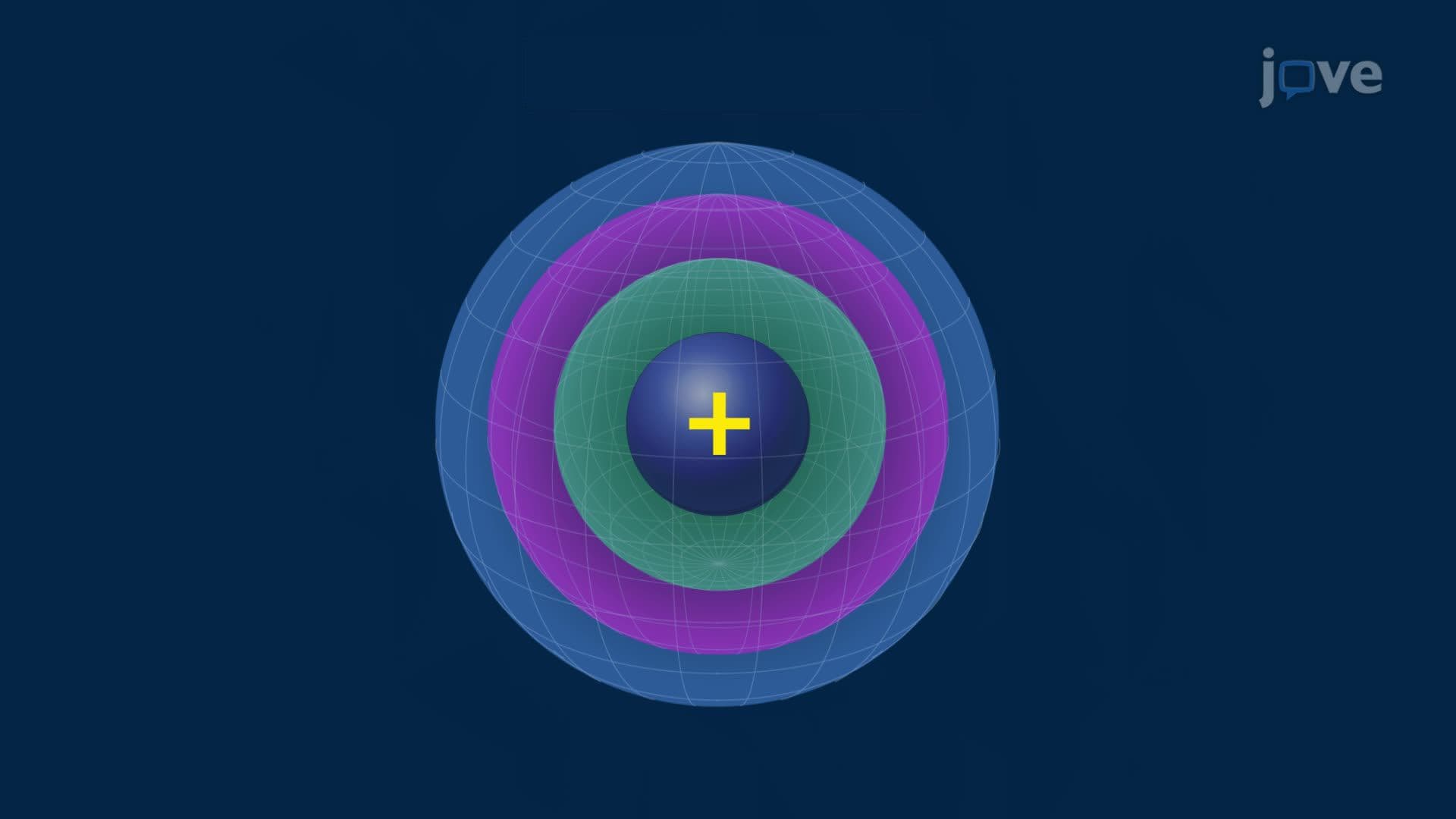
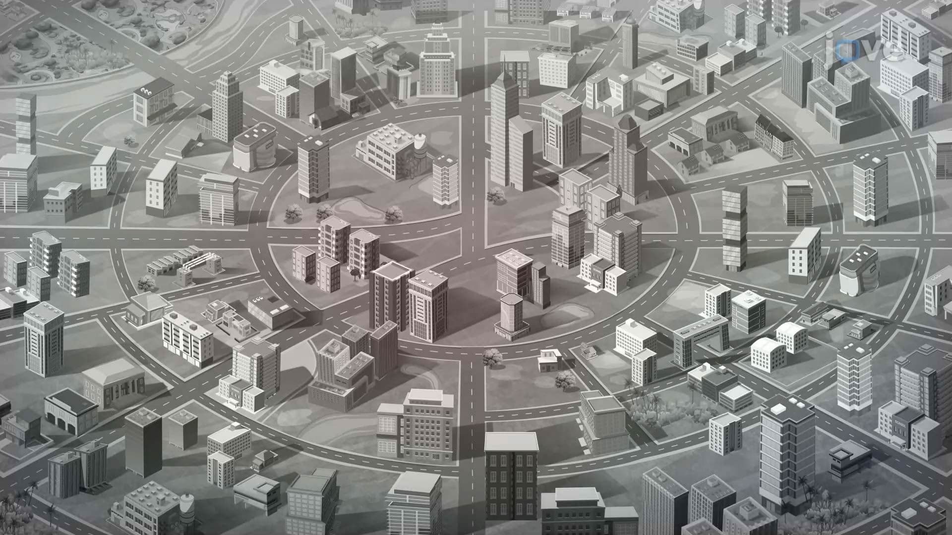
1. Functions of Two or More Variables and Their Graphs A multivariable function assigns exactly one output to every input pair, creating a surface in three-dimensional space. For example, traffic density across a US city corridor depends on both road position and time of day — two independent inputs producing one density value. Functions of three variables, such as electric potential around a charge, assign a scalar to every point in space. Visualizing these functions requires three-dimensional graphs, where the vertical axis encodes the output, and level surfaces or level curves capture sets of equal output values.

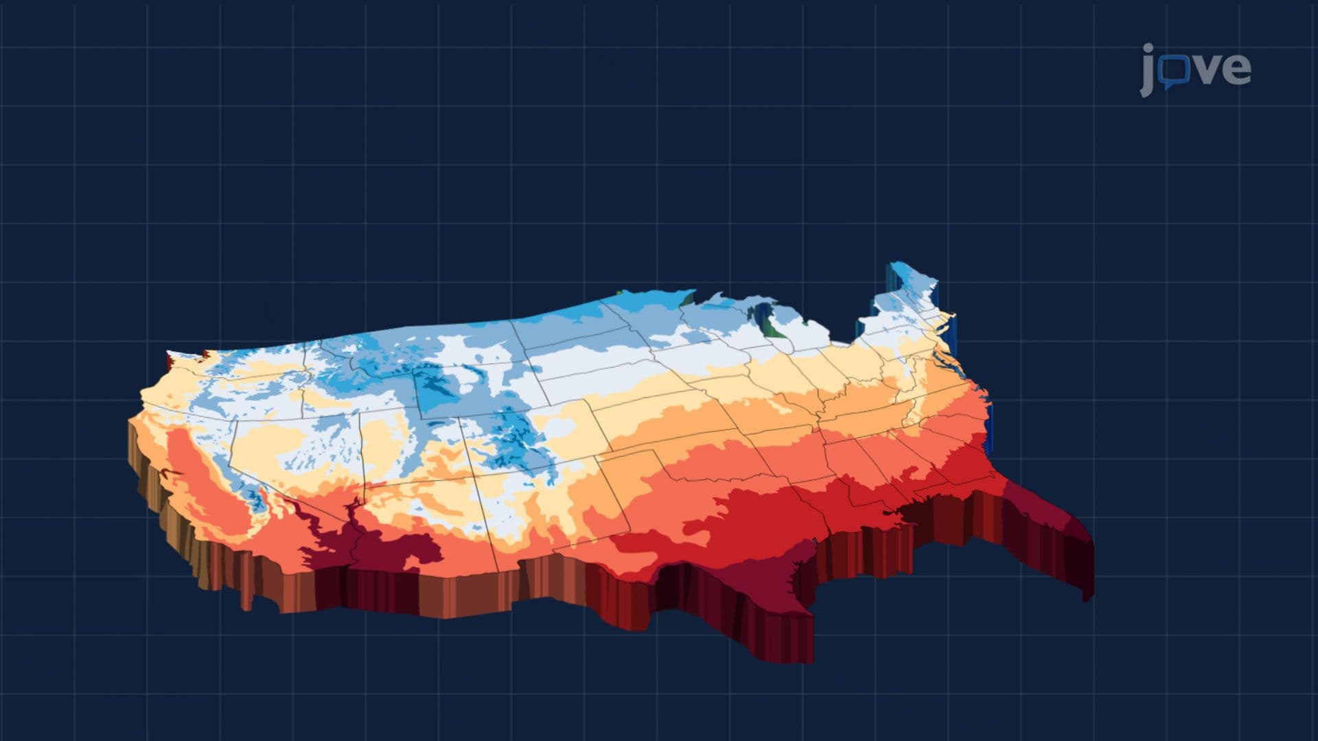
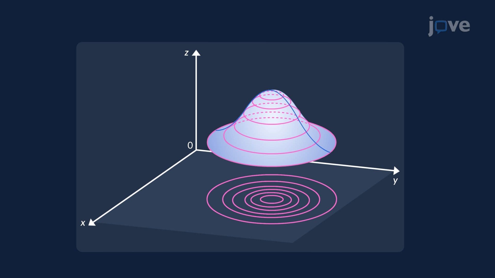
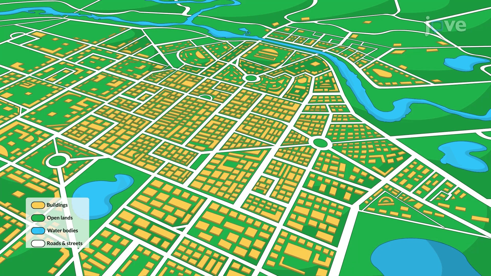
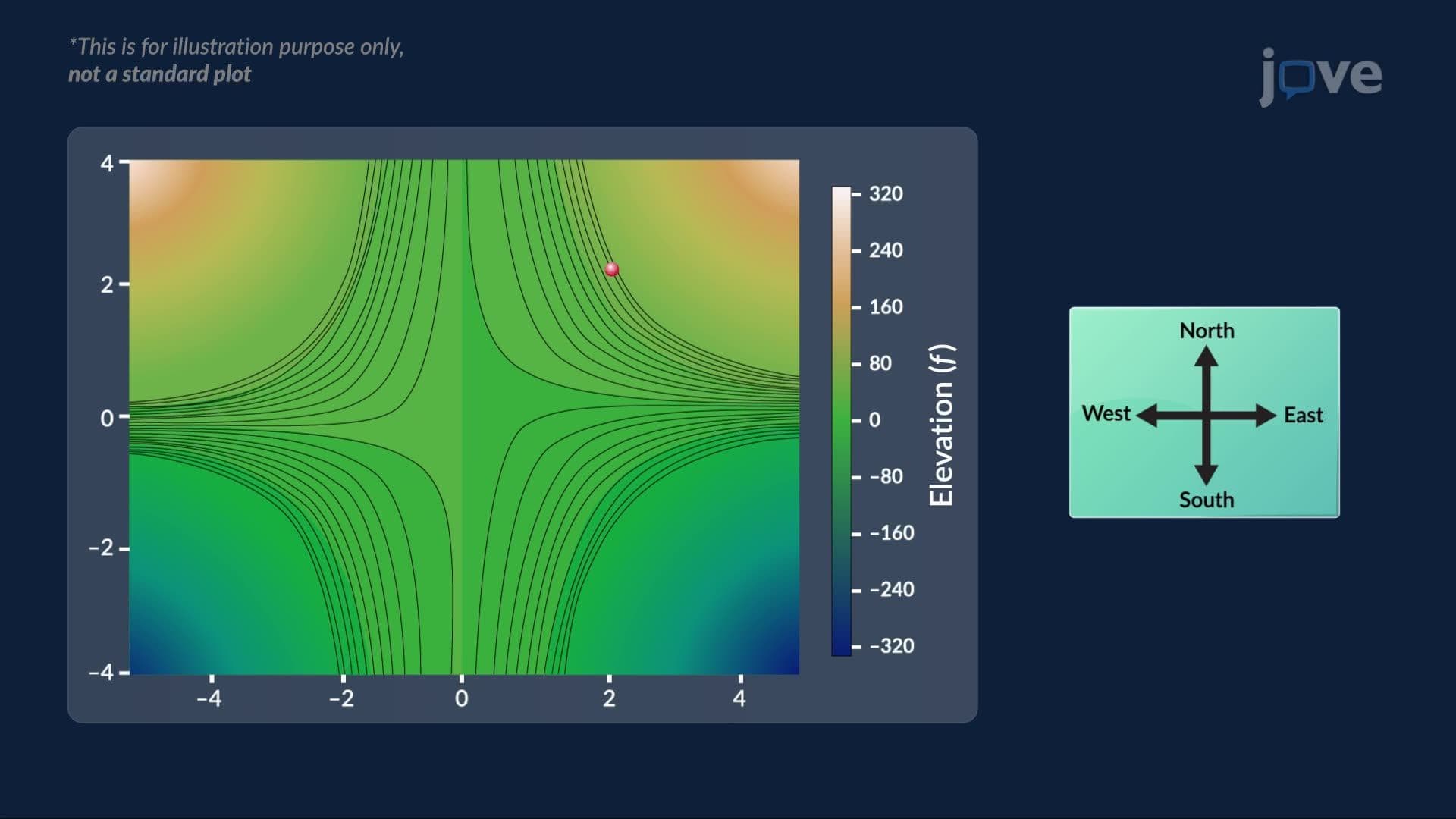
2. Level Curves, Contour Maps, and Level Surfaces Slicing a three-dimensional surface at constant heights produces level curves — familiar from US topographic maps published by the USGS. Each curve connects all input points sharing the same output value. Tightly spaced contour lines signal steep terrain; widely spaced lines indicate gentle slopes. For functions of three variables, the equivalent objects are level surfaces, such as the spherical equipotential surfaces surrounding an electric charge. Both tools transform invisible three-dimensional behavior into readable two-dimensional or geometric representations.

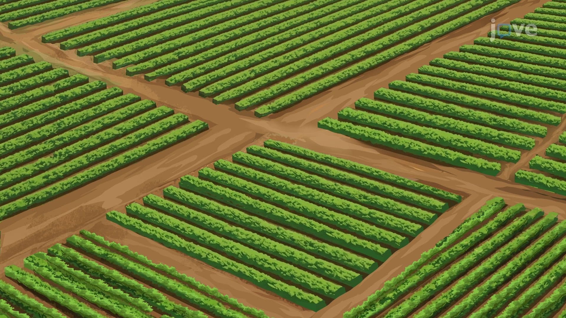
3. Limits and Continuity in Multivariable Calculus A limit of a multivariable function exists only when the function approaches the same value along every possible path toward the target point — a stricter requirement than in single-variable calculus. Standard limit laws, including the sum and difference laws, extend naturally to multivariable settings. Continuity requires that the function be defined at a point, that its limit exist, and that the two values agree. In precision agriculture applications across the US Midwest, continuous soil-moisture models ensure gradual, predictable field variation that guides efficient irrigation decisions.

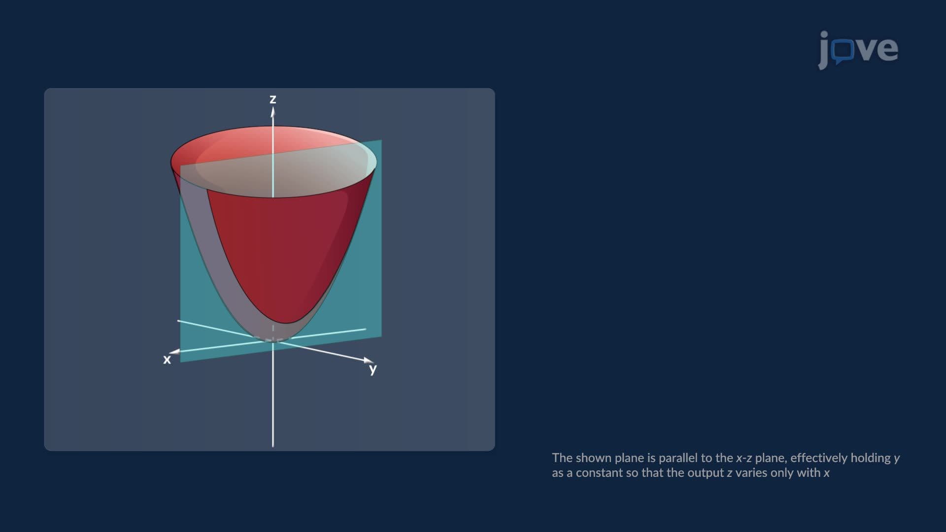
4. Introduction to Partial Derivatives and Their Interpretations A partial derivative measures how a function changes when one input varies while all others are held fixed. For a production function P(T, M) — where T represents labor and M represents machine capacity in a US manufacturing plant — the partial derivative with respect to T reveals how much output increases per additional labor unit, holding equipment constant. Geometrically, intersecting the surface with a vertical plane parallel to one axis produces a curve, and the partial derivative equals the slope of that curve's tangent line at the chosen point.

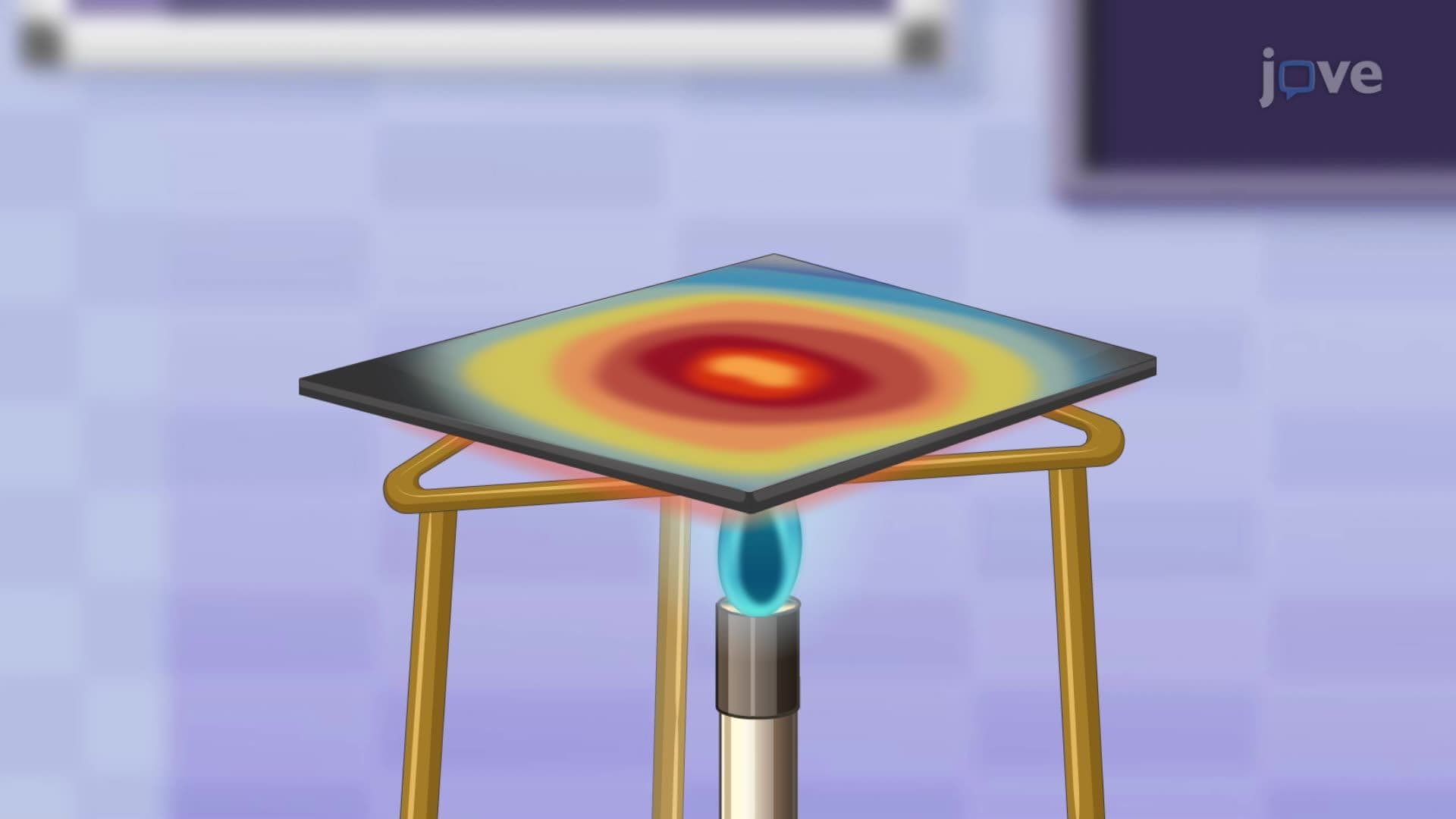
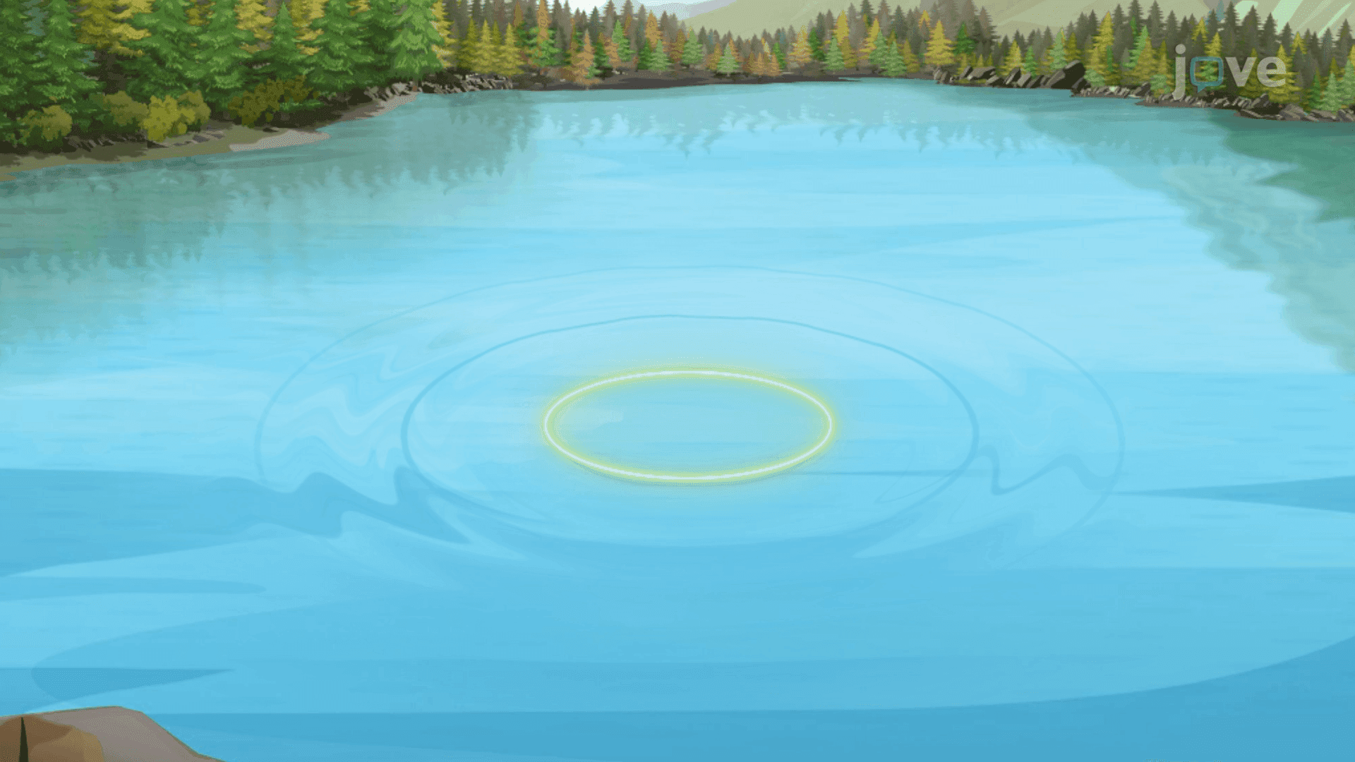
5. Higher-Order Partial Derivatives and Partial Differential Equations Differentiating a partial derivative again yields second-order derivatives. Pure second-order derivatives measure curvature along a single axis, while mixed partial derivatives capture how the rate of change in one direction is influenced by movement in another — revealing a geometric "twist" in the surface. These higher-order derivatives appear directly in partial differential equations (PDEs), which govern physical phenomena such as wave propagation across water, heat distribution through metal plates, and signal transmission in US telecommunications infrastructure. PDEs connect spatial and temporal changes through a single governing equation.

6. Tangent Planes and Linear Approximations At any smooth point on a surface, the two first-order partial derivatives define slopes along perpendicular cross-sections. The tangent plane passes through those two tangent lines simultaneously, forming the best local flat approximation to the curved surface. Linear approximation exploits this flatness: near a known monitoring location — such as an air-quality sensor station in Los Angeles — the pollution concentration at a nearby coordinate can be estimated using the tangent plane equation rather than the full curved model. Accuracy decreases as the estimation point moves farther from the reference location.

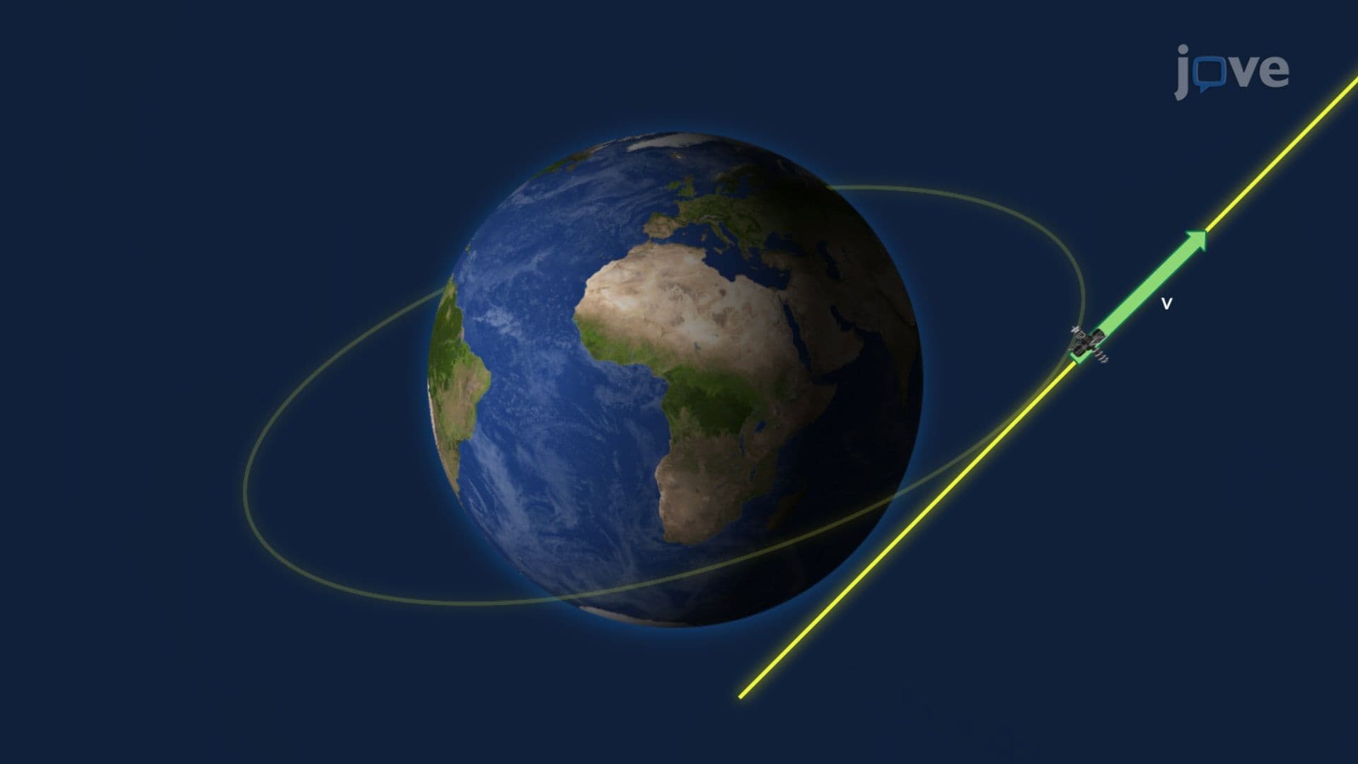
7. The Multivariable Chain Rule and Implicit Differentiation When an output depends on intermediate variables that each depend on a common parameter, the multivariable chain rule decomposes the total rate of change into a sum of partial contributions. A weather balloon rising through the atmosphere changes temperature because both altitude and humidity shift over time — the chain rule combines both contributions precisely. Implicit differentiation with partial derivatives extends this to equations where one variable is defined implicitly by another, such as a satellite's circular orbit equation, revealing instantaneous velocity direction without ever isolating the dependent variable explicitly.

8. Directional Derivatives and the Gradient Vector Partial derivatives measure slopes only along axis-parallel directions, but a hiker on a US mountain trail moves in any arbitrary direction. The directional derivative quantifies the rate of elevation change along any chosen direction, expressed using a unit vector. The gradient vector assembles both first-order partial derivatives into a single vector pointing in the direction of steepest ascent. Its magnitude measures how steep that ascent is. The directional derivative achieves its maximum value exactly when the movement direction aligns with the gradient — a result proven using the dot product and cosine relationship.

9. Gradient Vectors: Geometric Significance and Tangent Planes to Level Surfaces On a level surface — where the function output stays constant — every curve lying on the surface has a tangent vector perpendicular to the gradient. This perpendicularity, derived from the chain rule, establishes the gradient as the normal vector to the tangent plane at that point. A hiker walking at constant altitude moves perpendicular to the gradient, which always points directly uphill. In civil engineering applications, road gradient values directly influence vehicle fuel efficiency and speed ratings, making this geometric interpretation practically essential for US highway design standards.

10. Local Extrema, Critical Points, and Lagrange Multipliers Local maxima and minima of multivariable functions occur at critical points, where both partial derivatives equal zero and the tangent plane is locally flat. Finding extrema under constraints — maximizing the volume of an open cardboard box built from a fixed area of material, or minimizing the surface area of a shipping carton at a fixed volume — requires Lagrange multipliers. This method finds the point where the gradient of the objective function is parallel to the gradient of the constraint, introducing a proportionality constant lambda. Problems with two simultaneous constraints extend the method by introducing a second multiplier, systematically solving complex real-world optimization scenarios.