Loading subject page…

92 views

Video Summary: Level Curves and Contour Maps Explained
Ever wonder how hikers navigate mountains using just a flat paper map? Level curves and contour maps make that possible, and they're one of the most powerful ideas in multivariable calculus. The US Geological Survey uses contour maps to chart terrain across national parks like Yellowstone. Each line represents a constant elevation, turning complex 3D surfaces into readable 2D maps. Watch the full video on JoVE Coach to master this concept with expert-led visuals and step-by-step explanations.
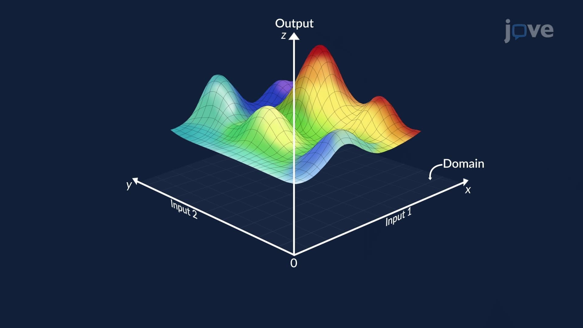
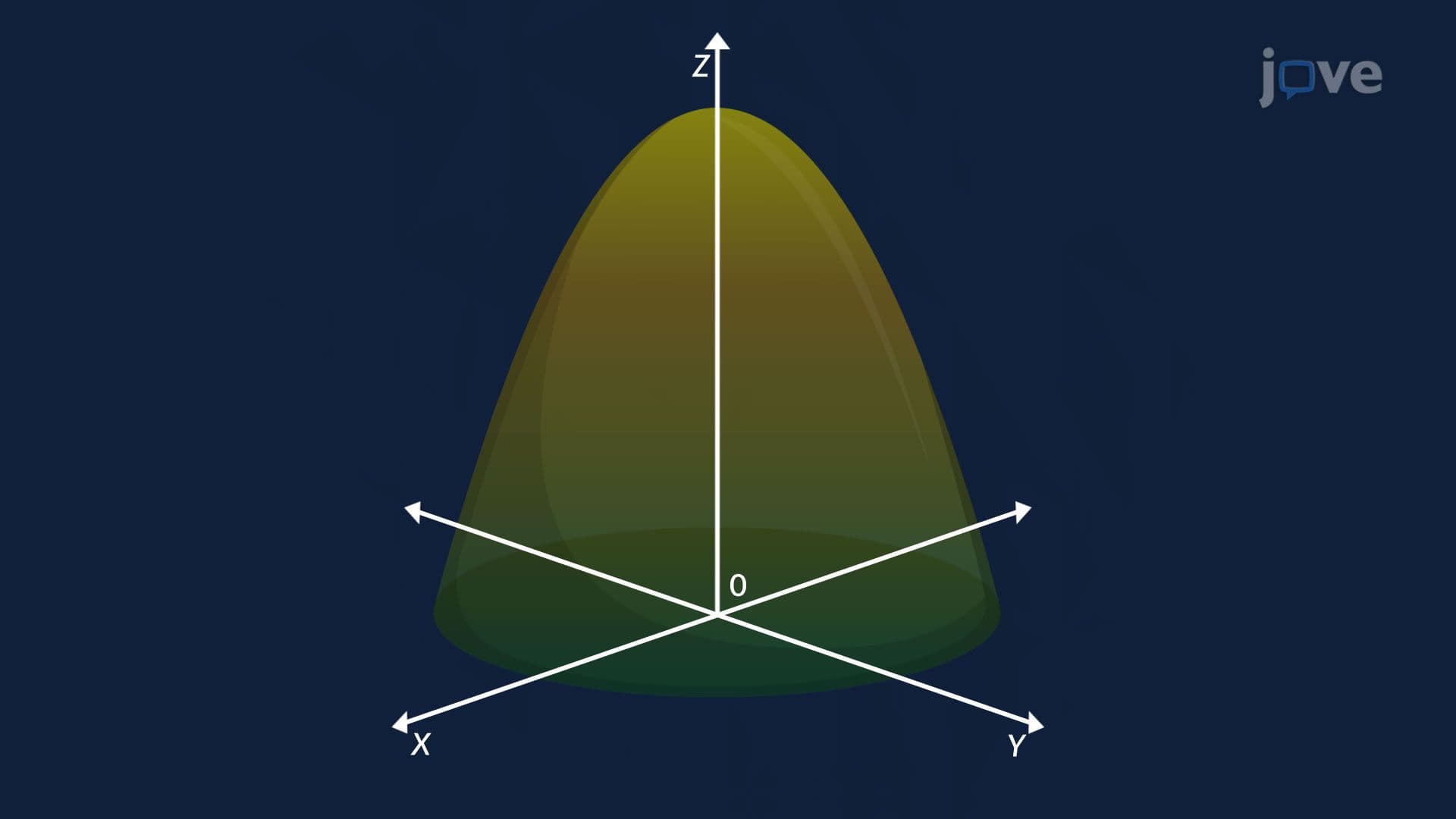
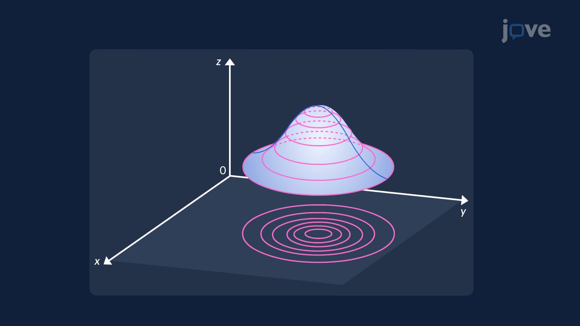
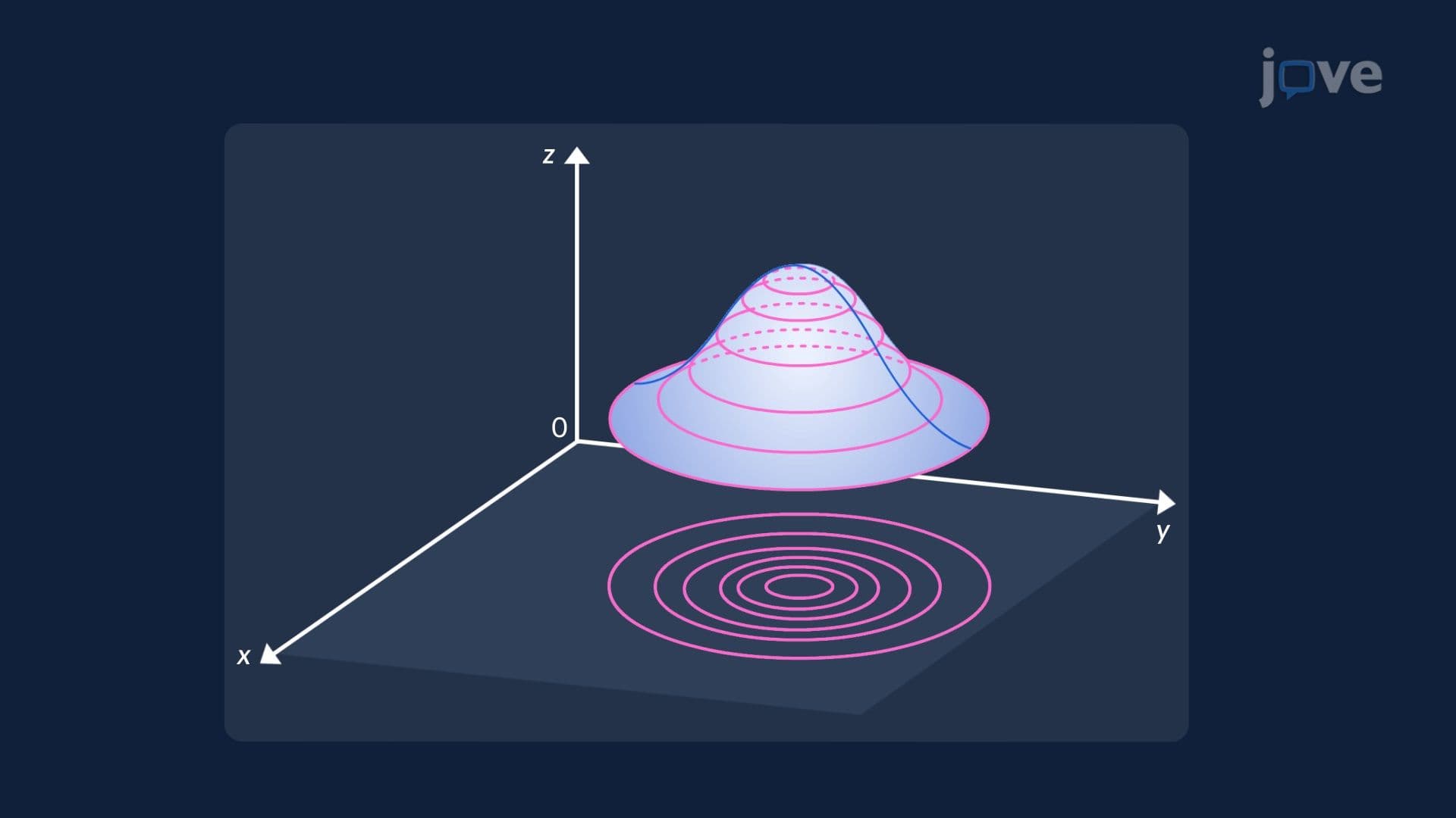
In multivariable calculus, a surface is described by a function of two variables, written as z = F(x, y). Visualizing this surface in three dimensions can be challenging, which is exactly where level curves and contour maps become essential tools. A level curve, also called a contour line, is the collection of all points (x, y) in the xy-plane where the function equals a fixed constant: F(x, y) = k. By computing level curves for several values of k, you build a contour map: a flat, two-dimensional diagram that encodes the full shape of a three-dimensional surface.
Imagine slicing a mountain-shaped surface with a series of horizontal planes at evenly spaced heights, say, every 500 feet. Each plane intersects the surface in a closed curve. When all of those curves are dropped straight down onto the flat xy-plane, they form a contour map. The result is exactly what the US Geological Survey (USGS) produces for wilderness areas across the country. Hikers in the Rocky Mountains or Appalachian Trail use these maps to estimate how difficult a climb will be before ever setting foot on the trail.
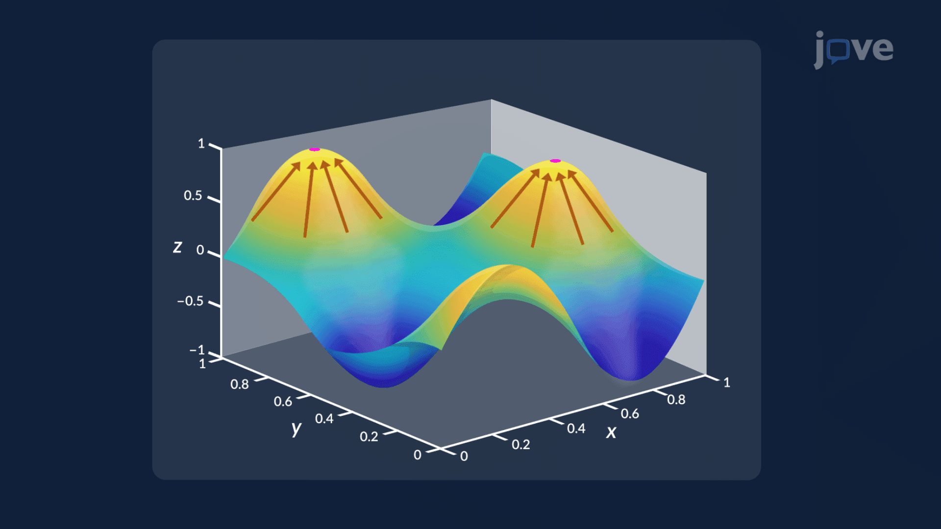
One of the most practical skills contour maps teach is how to read slope visually. When contour lines are crowded close together, the surface is rising or falling steeply, like a cliff face. When lines are spread far apart, the terrain is nearly flat. This relationship between line spacing and slope directly previews more formal calculus concepts like directional derivatives and the gradient vector. The gradient at any point on a surface always points in the direction of steepest ascent and is always perpendicular to the level curve passing through that point, a geometric insight tested frequently in college-level calculus courses.
Level curves appear across multiple academic contexts. In AP Calculus BC and first-year college calculus courses at universities like MIT OpenCourseWare's 18.02 (Multivariable Calculus), students are expected to sketch level curves and match them to given surfaces. In MCAT preparation, contour-style reasoning appears in physics passages involving potential energy surfaces. Understanding level curves also lays the groundwork for more advanced ideas: tangent planes approximate surfaces near a point, higher-order partial derivatives describe curvature, and finding maximum and minimum values of functions of two variables often involves analyzing where level curves change shape or spacing.
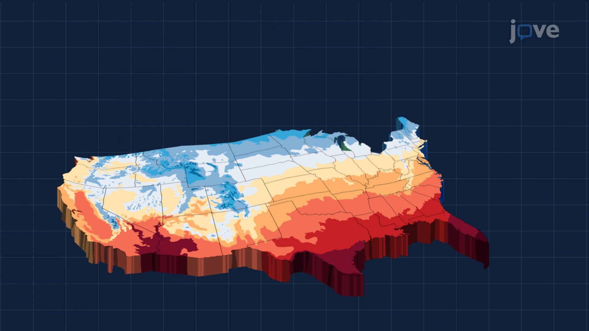
Weather forecasting relies on contour maps of atmospheric pressure, isobars on a weather chart are level curves of a pressure function. Financial analysts use similar tools to visualize risk surfaces. Even in medicine, MRI software generates "contour slices" of tissue at fixed depths. Mastering this concept early in your calculus journey gives you a visual and mathematical framework that pays dividends across STEM disciplines.
Related Micro-courses