Loading video…

 24 Concepts
 93 views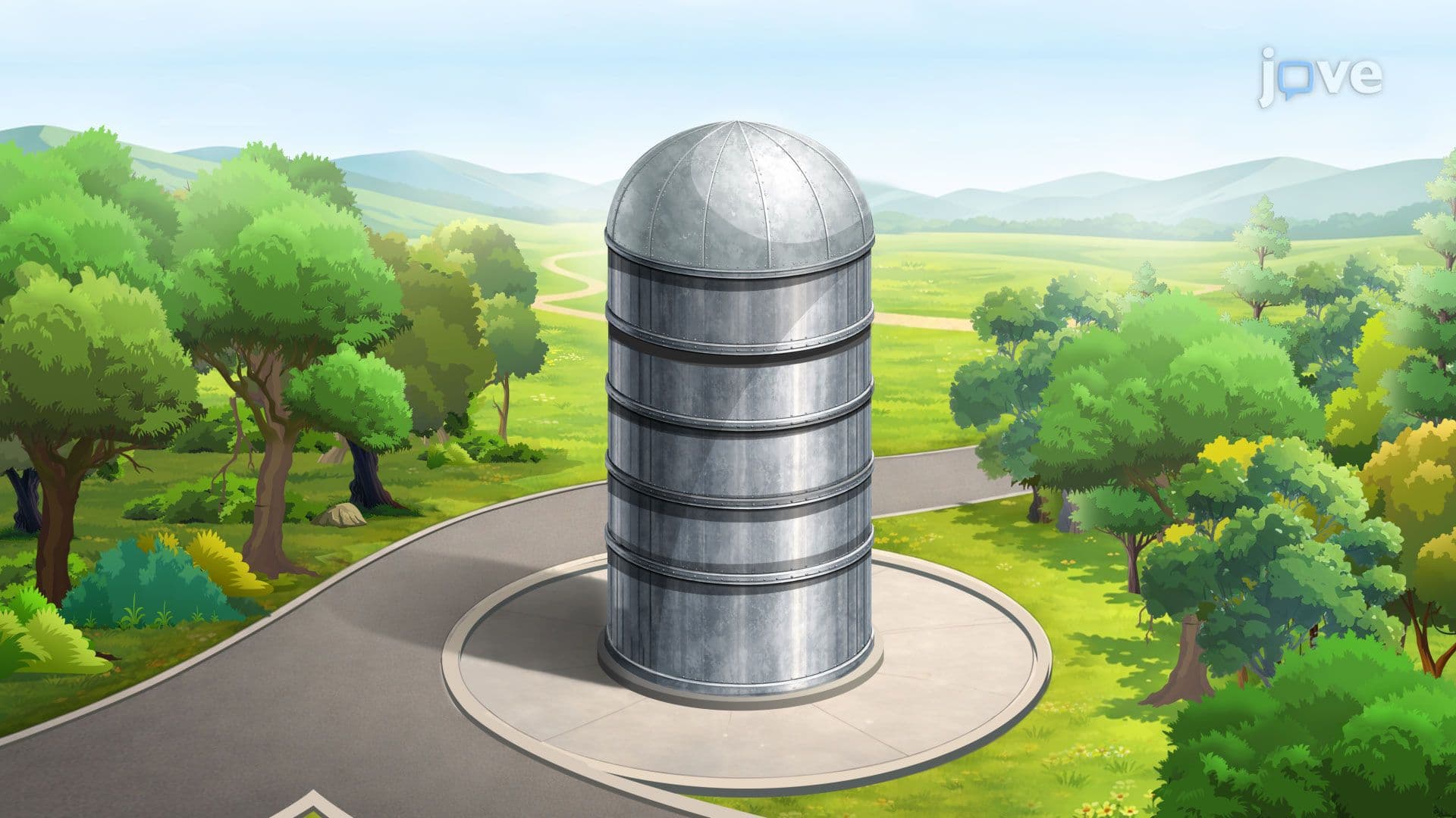

Video Summary: Problem Solving in Lagrange Multipliers
How do engineers design grain silos that hold the most grain while using the least amount of steel? The answer lies in problem solving in Lagrange multipliers, a powerful calculus technique for optimizing real-world systems under constraints. This concept, known as Problem Solving in Lagrange Multipliers, shows how maximizing a silo's volume with fixed surface area leads to a clean geometric result: the optimal cylinder height equals its radius. Watch the full video on JoVE Coach to master this concept with expert-led visuals and step-by-step explanations.
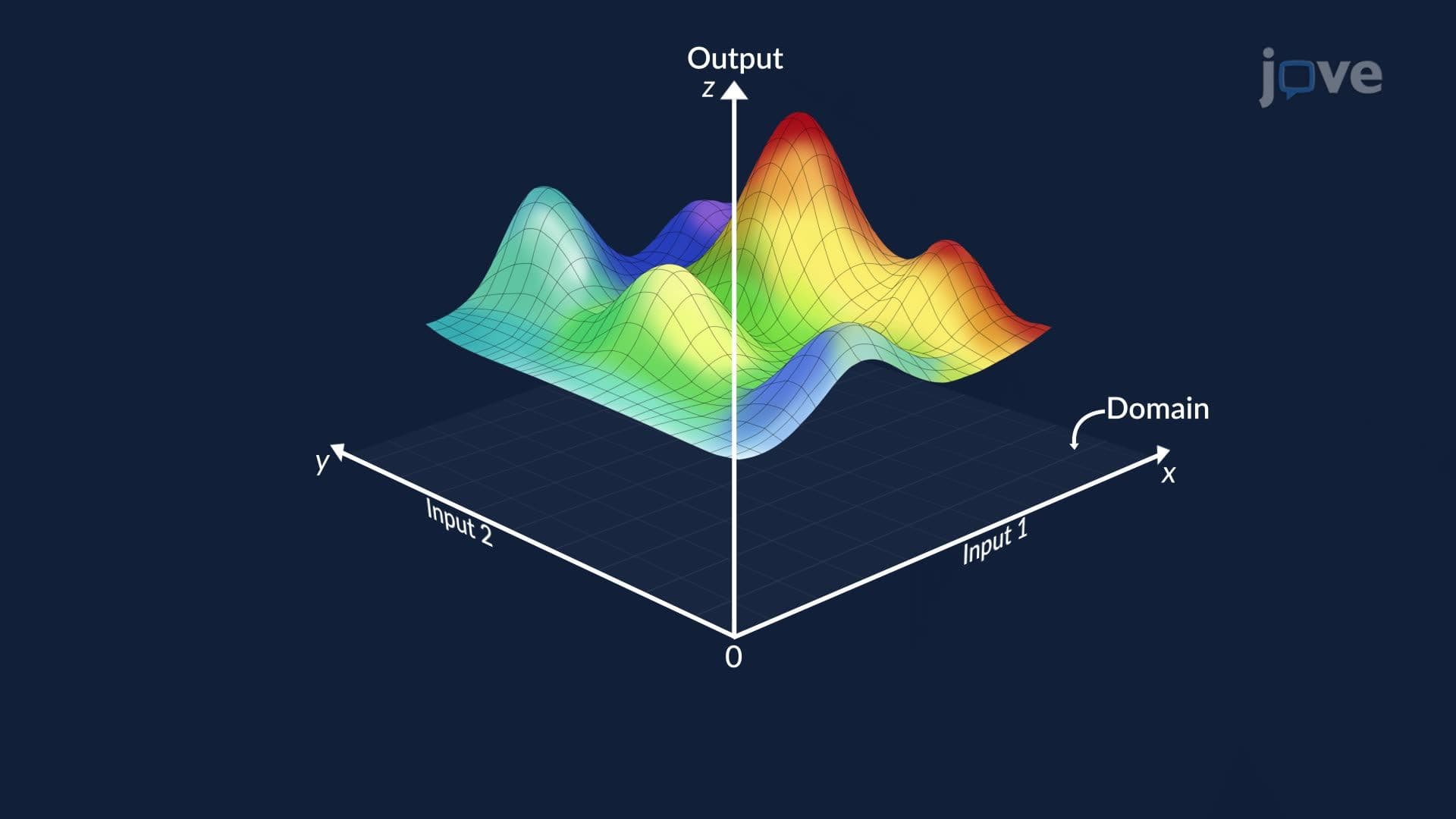
Optimization is one of the most practical skills in mathematics, but real-world problems rarely come without restrictions. You cannot simply minimize cost without a budget, or maximize volume without a material limit. Problem solving in Lagrange multipliers is the calculus framework that handles exactly this situation, finding the best possible outcome for a function when one or more constraints must be satisfied simultaneously. Developed by the 18th-century mathematician Joseph-Louis Lagrange, this method is a cornerstone of multivariable calculus courses taught at universities across the United States, from MIT to state university systems everywhere.
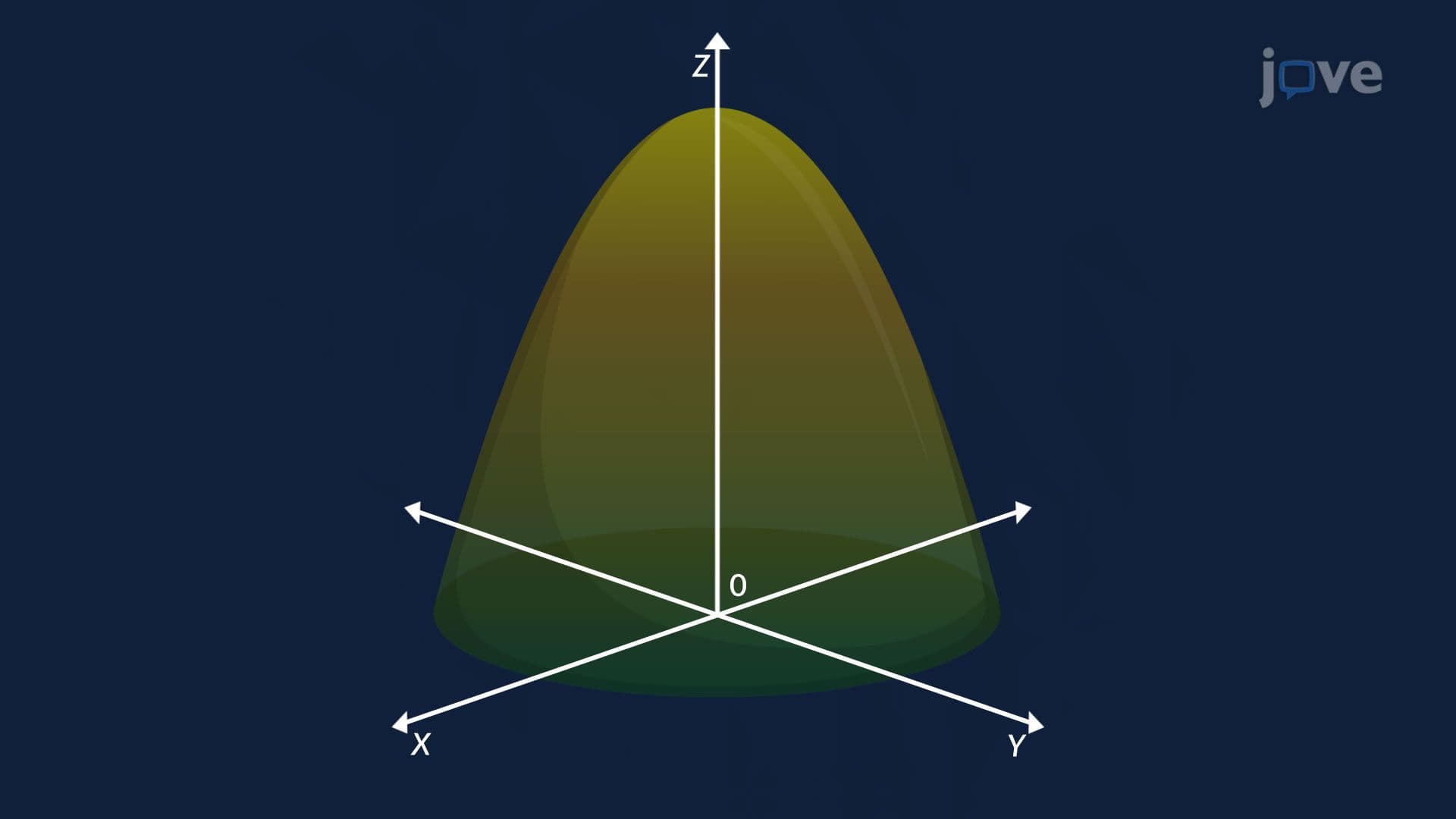
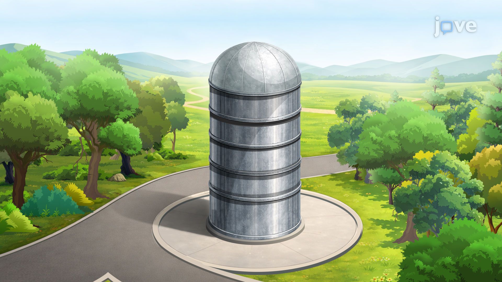
Every Lagrange multiplier problem begins with two key ingredients: an objective function (the quantity you want to optimize) and a constraint equation (the condition it must satisfy). For example, in a silo design problem, the objective function is the total volume V, expressed in terms of the cylinder's base radius r and height h, which includes both the cylindrical body and the hemispherical roof. The constraint is the fixed total surface area S, which accounts for the flat circular base, the lateral surface of the cylinder, and the curved hemispherical cap.
The Lagrange condition states: ∇V = λ · ∇S, where ∇ represents the gradient operator. This elegant equation says that at the optimal point, the gradient of the volume function must be parallel to the gradient of the surface area function. In practice, this generates one partial derivative equation for each variable, plus the original constraint, forming a complete system of equations to solve.
Once the gradient condition is written out, the next step is differentiating with respect to each independent variable. Differentiating with respect to h yields a straightforward expression for λ in terms of r. Substituting that expression into the equation obtained by differentiating with respect to r then creates a single equation relating h and r.
This process relies directly on skills from multivariable calculus: computing partial derivatives, applying the chain rule for partial derivatives, and solving systems of nonlinear equations. For the silo example, the algebra resolves to a strikingly clean result, the maximum volume is achieved when the cylinder height h equals the base radius r. This outcome is not obvious by inspection; it emerges only through the structured logic of the Lagrange method, demonstrating why the technique is so valued in engineering design.
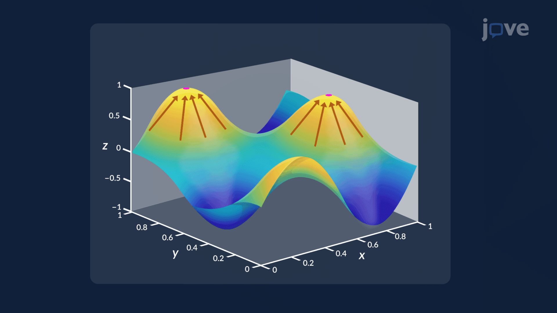
Understanding what is the geometric interpretation of the gradient vector helps make the Lagrange condition intuitive. The gradient of a function always points perpendicular to its level curves (or level surfaces in three dimensions). The Lagrange condition ∇V = λ · ∇S means the level surface of V is tangent to the constraint surface defined by S at the optimal point, the two surfaces just "kiss" without crossing. This is also closely related to directional derivatives: at the optimum, moving along the constraint produces no net change in the objective function, which is precisely the definition of a critical point under a constraint.
Problem solving in Lagrange multipliers is a standard topic in AP Calculus BC extensions, college-level Calculus III courses, and first-year engineering mathematics at US universities. It appears in economics coursework as utility maximization subject to a budget constraint, in chemical engineering for thermodynamic equilibrium problems, and in machine learning for constrained loss minimization. Students preparing for college midterms or final exams should practice identifying the objective function and constraint clearly before setting up the gradient equations, as setup errors are the most common source of lost points. Mastering higher-order partial derivatives and understanding maximum and minimum values of functions of two variables will also strengthen your foundation before tackling Lagrange problems.
Related Micro-courses