Loading subject page…

91 views

Video Summary: Continuity for Functions of Multiple Variables Explained
Did you know that a tiny break in a mathematical surface can make an entire irrigation model collapse? Continuity for functions of multiple variables ensures that a function's surface remains unbroken at every point, no holes, no jumps, no surprises. In US precision agriculture, farmers rely on continuous moisture models across fields to plan efficient irrigation. Watch the full video on JoVE Coach to master this concept with expert-led visuals and step-by-step explanations.
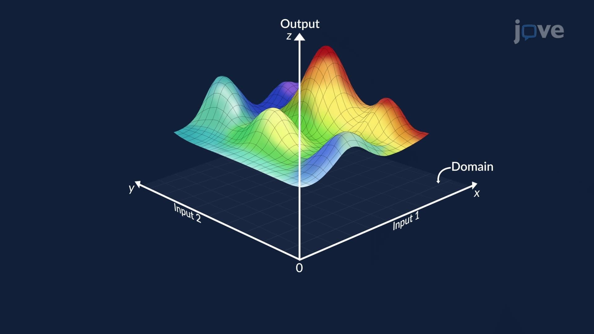
In single-variable calculus, a function is continuous when its graph has no breaks or holes. Continuity for functions of multiple variables extends that same intuition into higher dimensions, but with an important twist. Instead of approaching a point from just two directions (left or right), a function of two variables, f(x, y), must produce the same limiting value no matter which direction or path you use to approach a given point. That added complexity makes multivariable continuity both more powerful and more demanding to verify.
For a function f(x, y) to be continuous at a point (a, b), it must pass all three of the following conditions:
1. The function is defined at (a, b): f(a, b) must exist, no division by zero, no square root of a negative number, no undefined output. 2. The limit exists at (a, b): As (x, y) approaches (a, b) along every possible path, the function must converge to a single finite number. If two different paths yield two different values, the limit does not exist and continuity fails. 3. The limit equals the function value: lim(x,y)→(a,b) f(x, y) = f(a, b). The predicted value and the actual value must match exactly.
Failing even one condition means the function is discontinuous at that point, even if it looks "almost" continuous everywhere else.
One of the trickiest aspects of multivariable continuity, and a frequent source of exam errors, is path dependency. In single-variable calculus, you only check left-hand and right-hand limits. In multivariable calculus, you must confirm that the limit is the same along all paths: straight lines at any angle, parabolic curves, spirals, and more. A common exam strategy is to test two simple paths first (say, along y = 0 and y = x). If they give different values, the limit fails and the function is discontinuous. This concept is heavily tested in college-level Calculus III courses and appears in AP Calculus BC preparatory problem sets covering limit behavior.
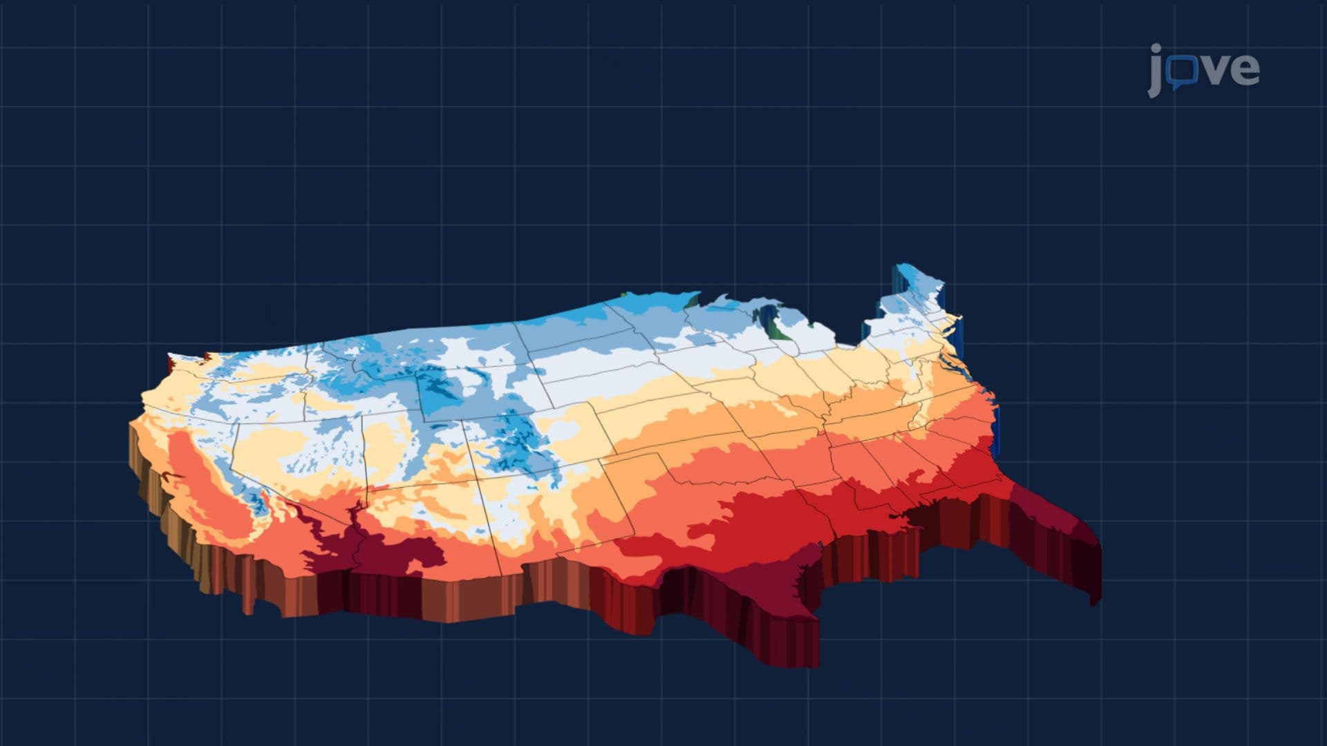
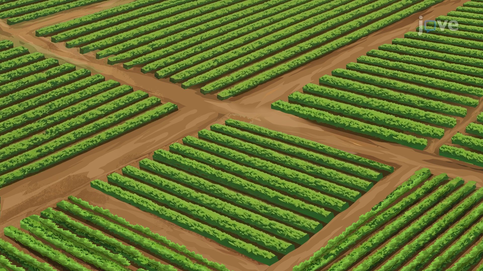
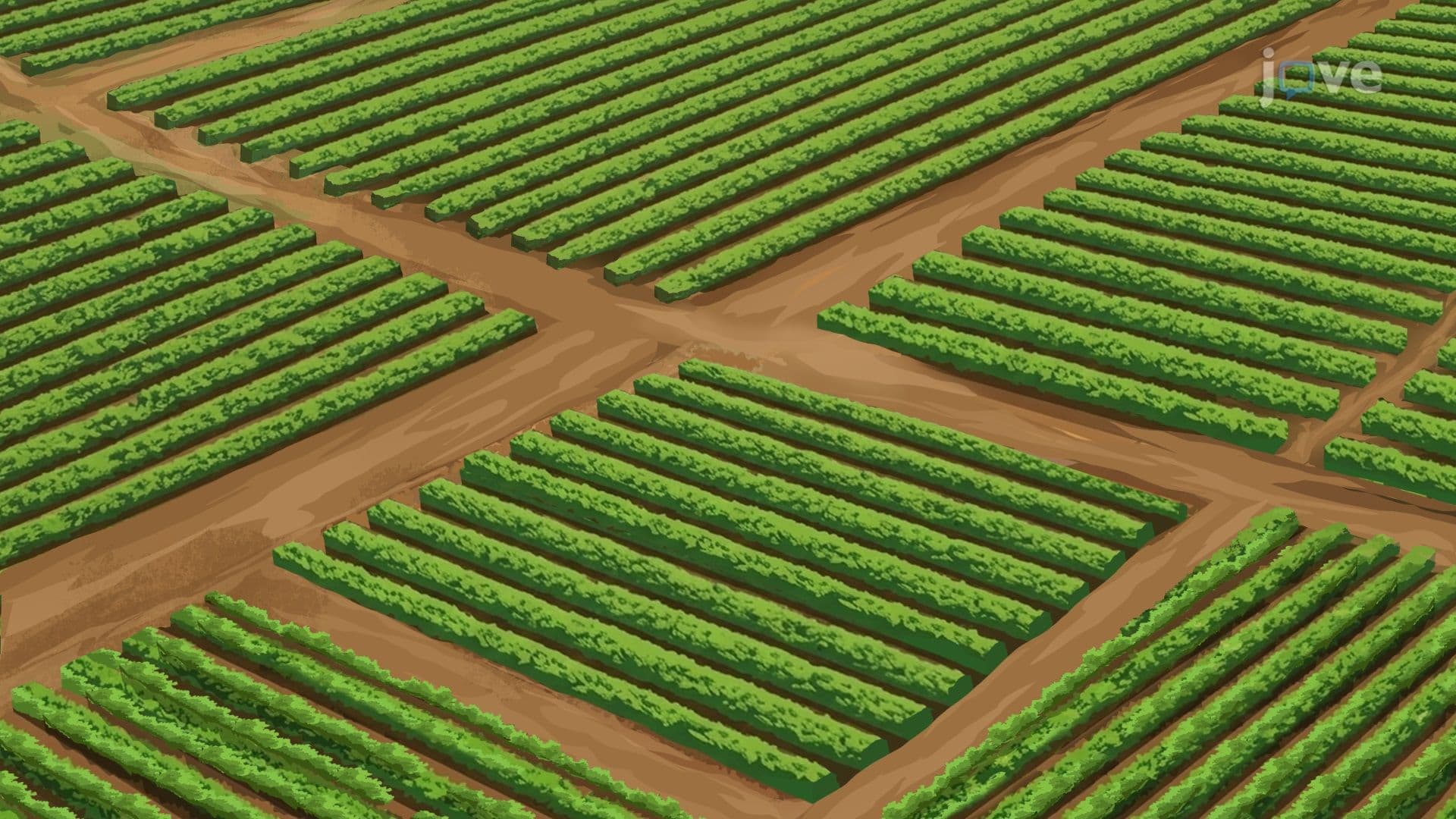
Continuity isn't just an abstract mathematical property, it has direct real-world relevance. In US precision agriculture, companies like John Deere and university extension programs at institutions such as Purdue and UC Davis use continuous mathematical models to map soil moisture across large fields. If the moisture function f(x, y) is continuous, moisture levels shift gradually, which allows irrigation systems to respond smoothly. A discontinuous model would suggest impossible sudden jumps in moisture, physically meaningless and operationally misleading.
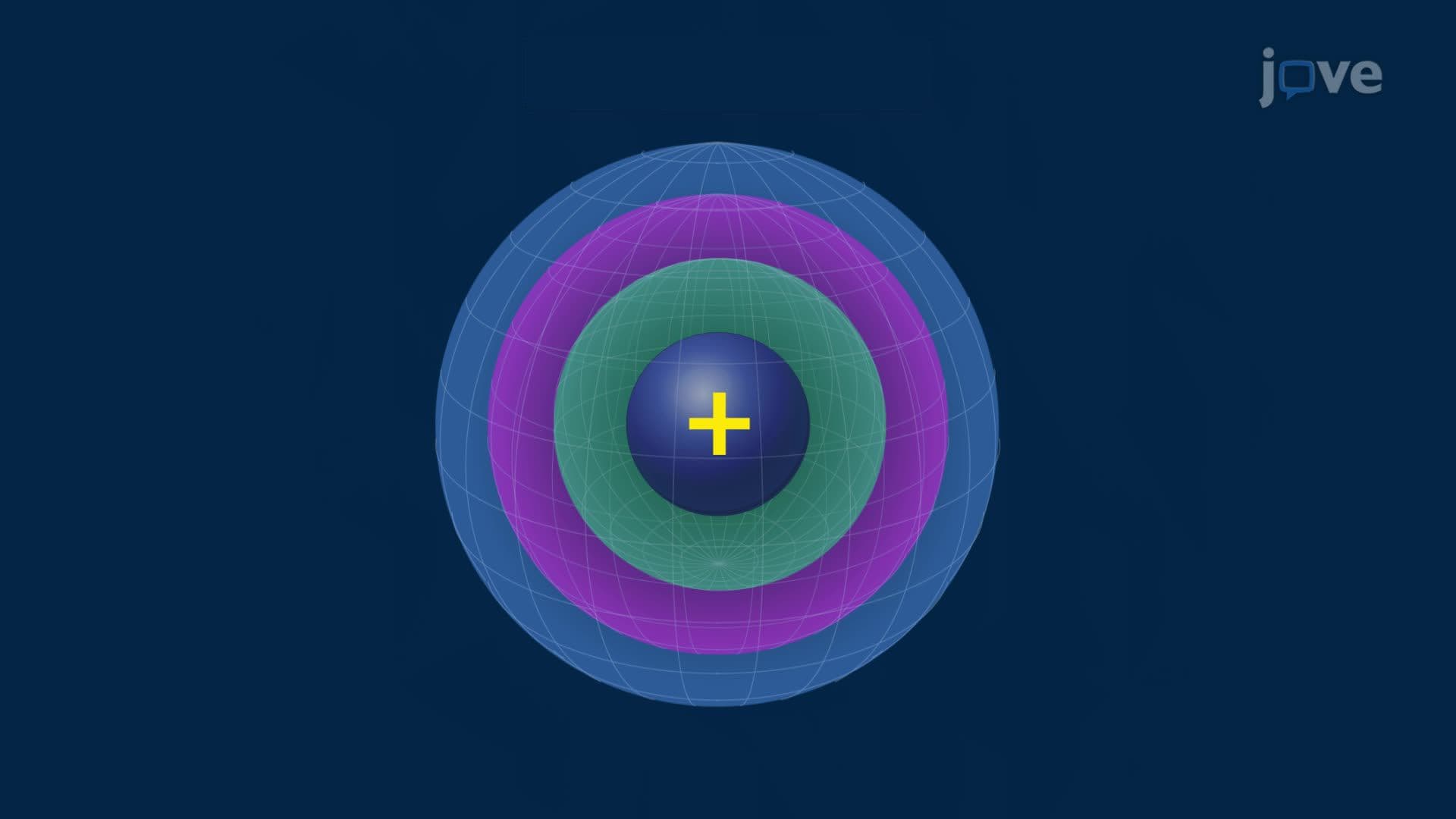
In engineering and physics, continuity underpins the behavior of temperature distributions, fluid pressure fields, and electromagnetic potential surfaces. Before you can apply tools like the gradient vector, directional derivatives, or tangent planes to a surface, that surface typically must be continuous, reinforcing why this foundational concept appears early in every multivariable calculus course.
Continuity serves as the gateway to virtually every advanced topic in multivariable calculus. Finding local extrema of a multivariable function requires continuity and differentiability on the domain. The chain rule for partial derivatives assumes continuity of the component functions. Higher-order partial derivatives are only guaranteed to be equal (Clairaut's Theorem) when the mixed partials are continuous. Understanding continuity now builds a strong scaffolding for optimization, gradient analysis, and surface modeling later in the course.
Related Micro-courses