Loading video…


 24 Concepts
 92 views

Video Summary: What are Directional Derivatives
Ever wondered how a hiker on a Rocky Mountain trail calculates the steepest path to avoid sliding? Directional derivatives solve exactly this problem. Unlike standard partial derivatives, which only measure slope along fixed x or y axes, directional derivatives measure the rate of change in *any* chosen direction across a surface. This makes them essential in multivariable calculus for modeling real terrain, fluid flow, and more. Watch the full video on JoVE Coach to master this concept with expert-led visuals and step-by-step explanations.
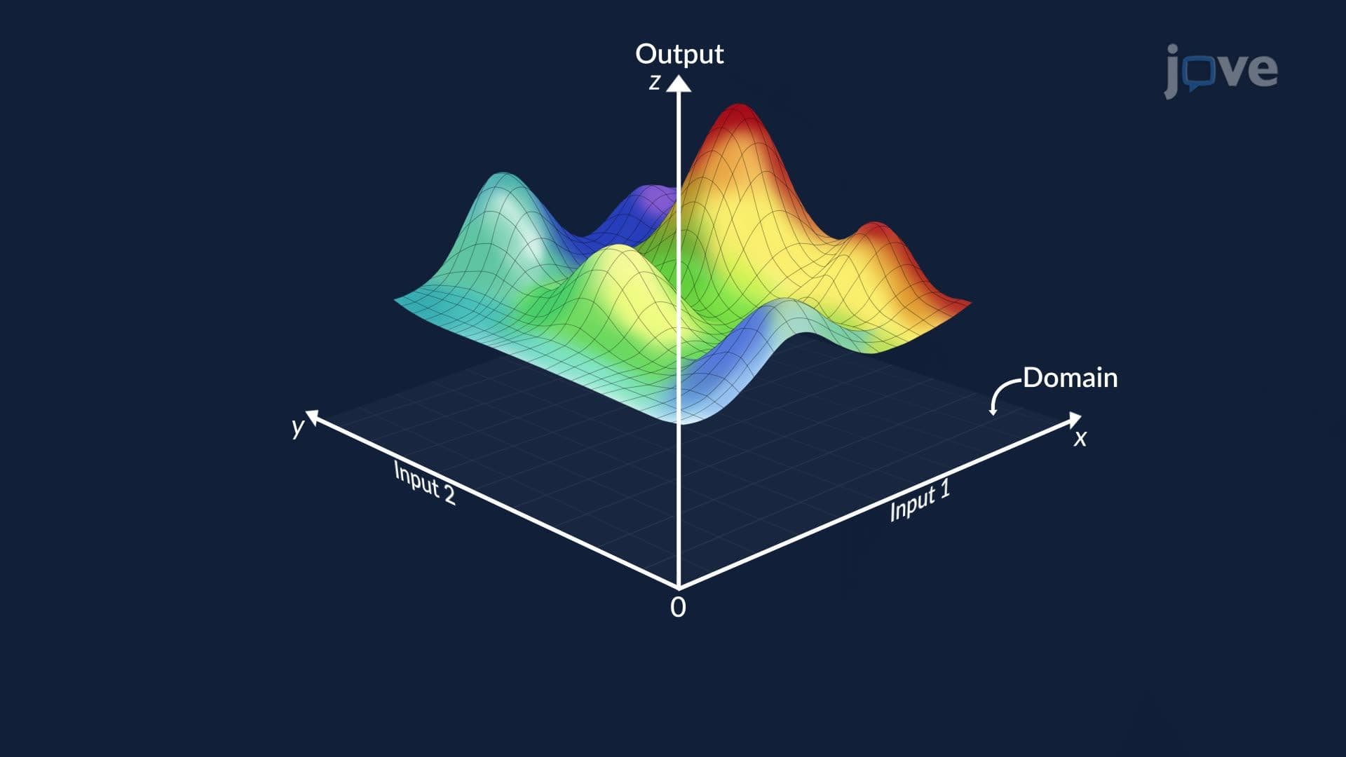
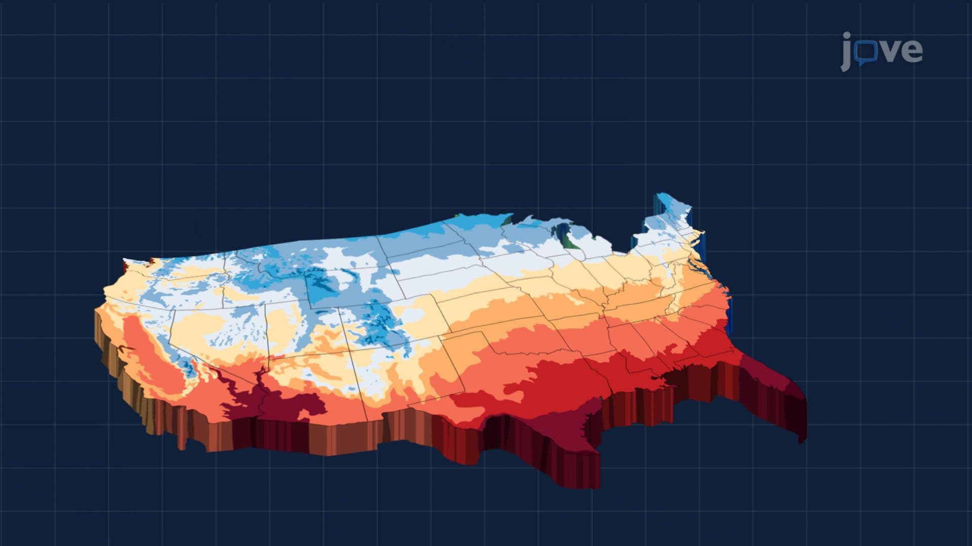
In single-variable calculus, a derivative tells you exactly how fast a function changes as you move along one dimension. But in the real world, think of a civil engineer mapping elevation changes across Yosemite Valley, or a meteorologist modeling temperature gradients across the Midwest, functions depend on *multiple* variables, and motion happens in *any* direction. This is precisely where directional derivatives become indispensable.
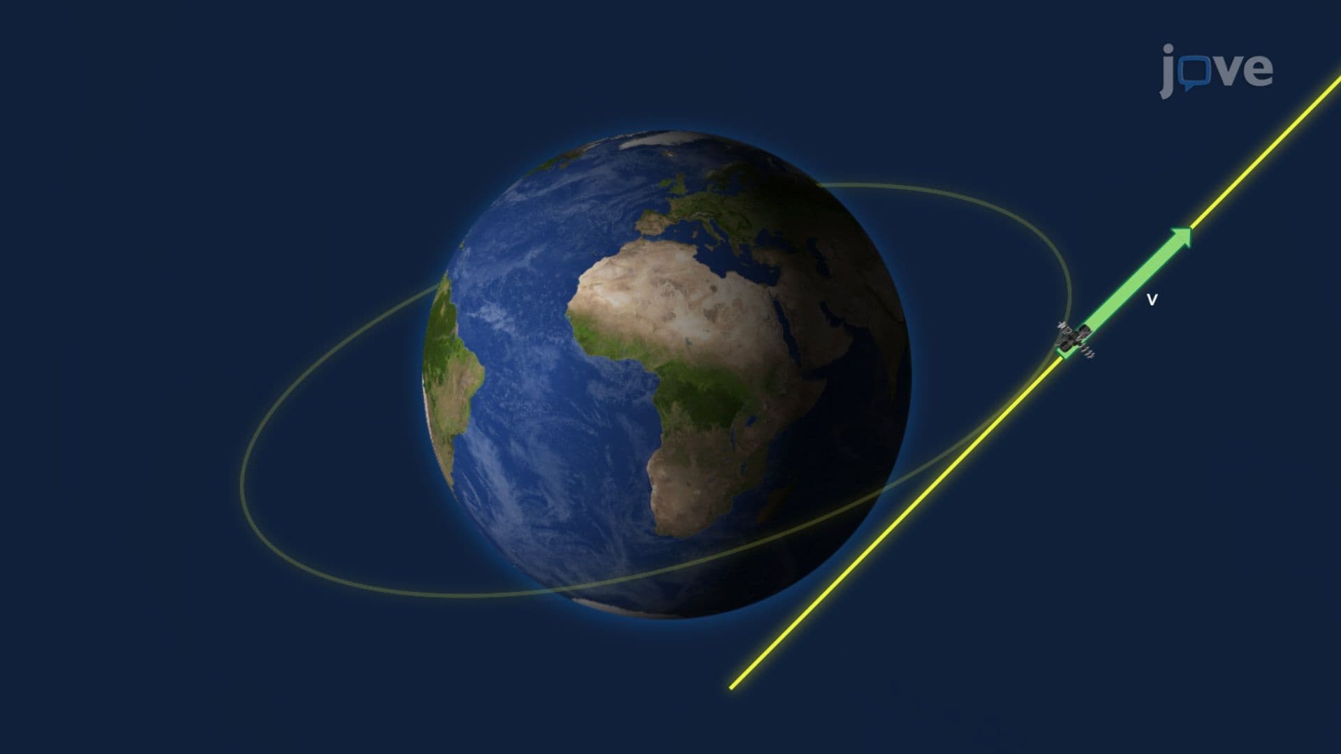
A directional derivative measures the instantaneous rate of change of a multivariable function as you move from a given point in a specific direction. Rather than being locked into the x-axis or y-axis, you can point in any direction across the input plane and ask: "How fast is this function changing as I head that way?"
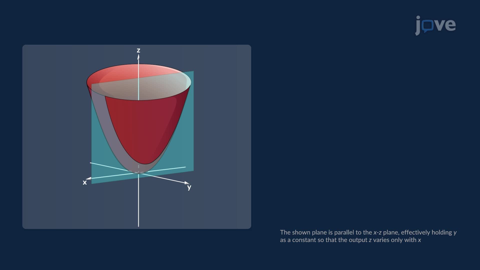
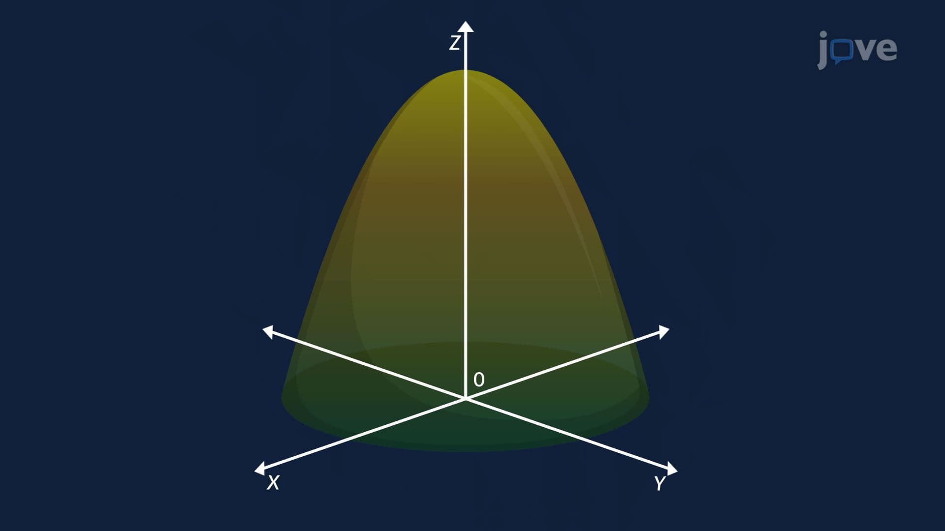
To appreciate directional derivatives, you first need to understand their building blocks: partial derivatives. For a function f(x, y), the partial derivative with respect to x, written as f(x), measures the slope of the surface in the direction parallel to the x-axis, holding y constant. Similarly, f(y) captures the slope parallel to the y-axis.
These are powerful but limited. They only sample two specific directions out of infinitely many possible ones. Real-world applications rarely confine motion to those two neat axes.
The key to unlocking any direction is the unit vector, written as u, with components (u_x, u_y). A unit vector has a magnitude of exactly 1, which ensures the directional derivative reflects the *rate* of change per unit of distance, not a distorted value caused by scaling.
For example, if you want to measure slope at a 45-degree angle northeast across a terrain model, your unit vector would be u = (1/√2, 1/√2). This vector precisely encodes the direction without inflating the result.
The directional derivative of f in the direction of unit vector u is calculated as:
D(u) f(x, y) = f(x) · u_x + f(y) · u_y
Here is what each part does:
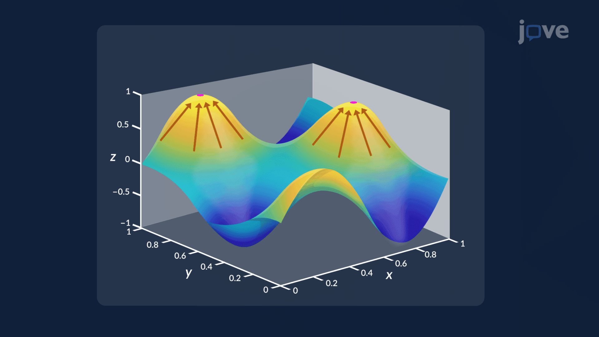
Notice that this formula connects directly to the dot product of the gradient vector ∇f = (f(x), f(y)) and the unit vector u. This elegant connection means the directional derivative is maximized when u aligns with the gradient, the gradient literally points "uphill" as steeply as possible. This insight drives optimization problems encountered in AP Calculus BC, college Calculus III courses, and real engineering applications.
In US college multivariable calculus courses, a standard requirement for STEM majors at universities like MIT, UC Berkeley, and Georgia Tech, directional derivatives appear in units covering gradient vectors, tangent planes, and the optimization of functions of two variables. On exams, students are often asked to find the directional derivative at a specific point, determine the direction of steepest ascent, or identify local extrema using second-order analysis.
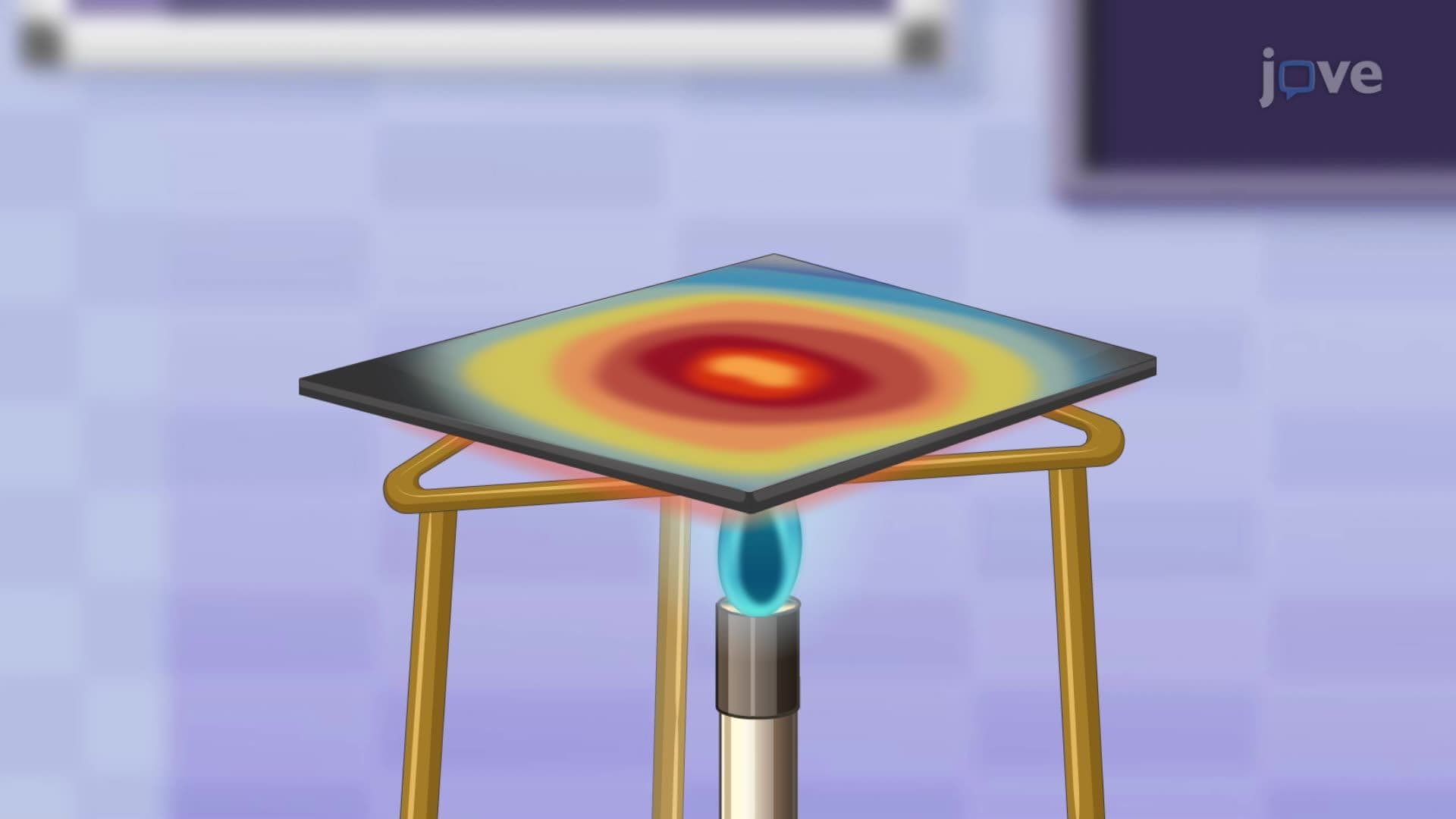
Beyond academics, directional derivatives model how heat spreads across a metal plate, how pressure changes in atmospheric science, and how machine learning algorithms follow gradients during neural network training. Understanding this concept is not just an academic exercise, it is a gateway to higher-level mathematical thinking used across engineering, physics, economics, and data science.
Related Micro-courses