Loading subject page…


92 views


Video Summary: Tangent Planes to Level Surfaces Explained
Ever wonder why a flat plane can perfectly describe a curved 3D surface at a single point? Tangent planes to level surfaces basics reveals exactly that, and it's more intuitive than you'd expect. Think of a hiker at Rocky Mountain National Park walking along a constant-elevation trail: the flat ground beneath their feet models the tangent plane. Watch the full video on JoVE Coach to master this concept with expert-led visuals and step-by-step explanations.
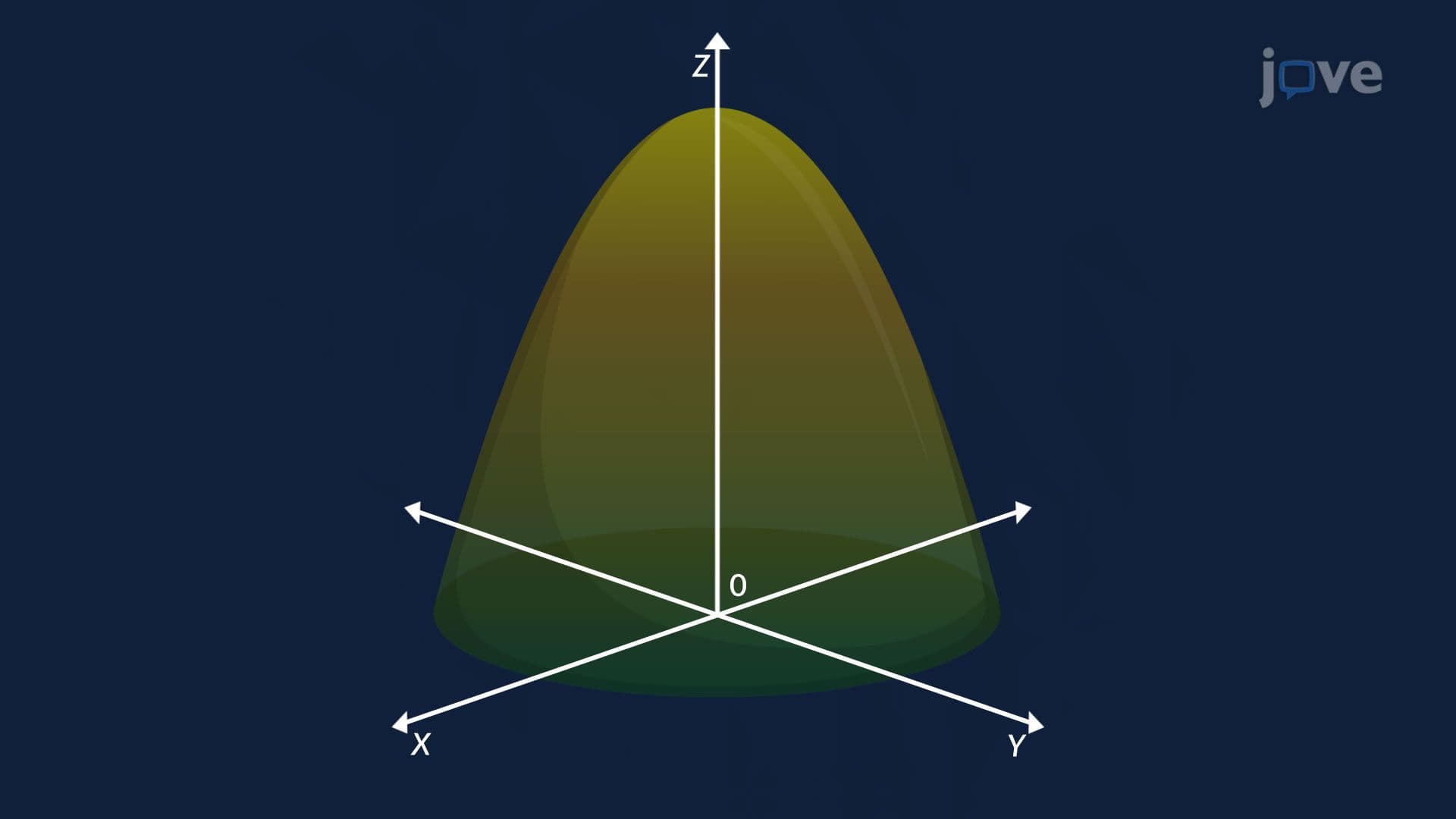
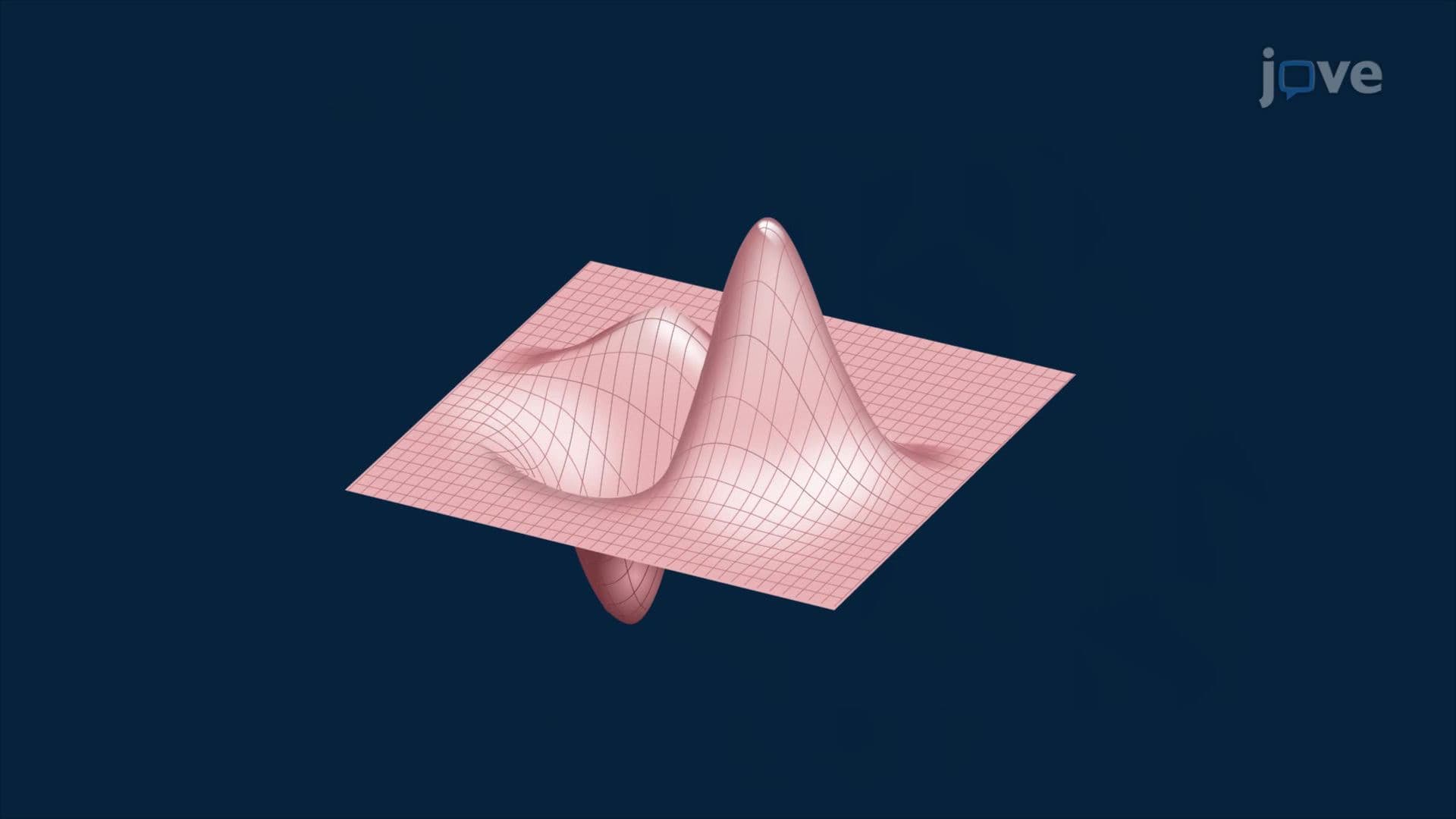
In single-variable calculus, a tangent line touches a curve at one point and approximates its behavior nearby. In multivariable calculus, this idea extends into three dimensions: a tangent plane touches a curved surface at a single point and approximates its local shape. Understanding tangent planes to level surfaces is one of the most important geometric skills in any college-level calculus course, and it appears across physics, engineering, and data science.
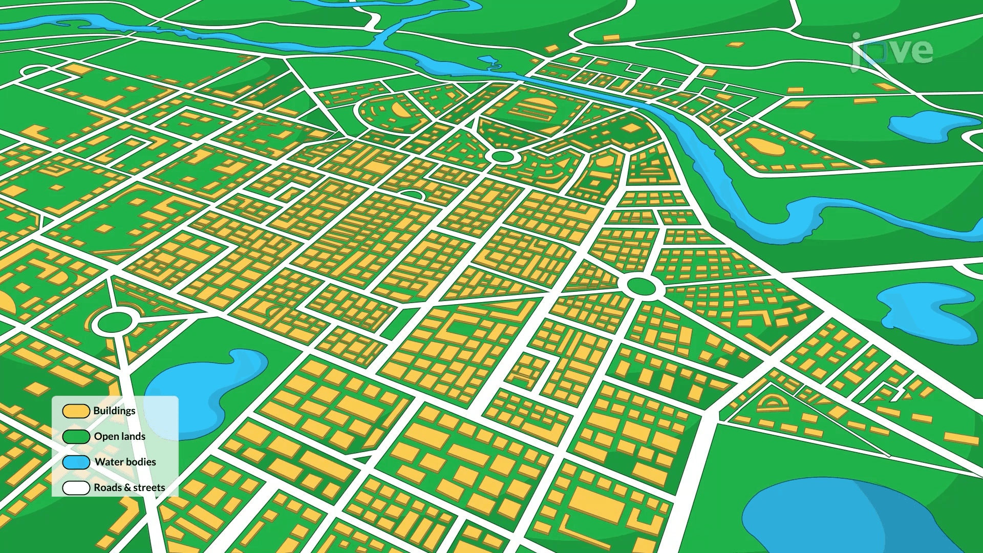
A level surface is the set of all points (x, y, z) in three-dimensional space where a function of three variables F(x, y, z) equals a fixed constant k. You can think of it as the 3D version of a contour line on a topographic map. For example, the surface of a sphere centered at the origin, x² + y² + z² = 25, is a level surface of F(x, y, z) = x² + y² + z². Engineers at firms like NASA use level surfaces to model pressure boundaries and thermal gradients around spacecraft.
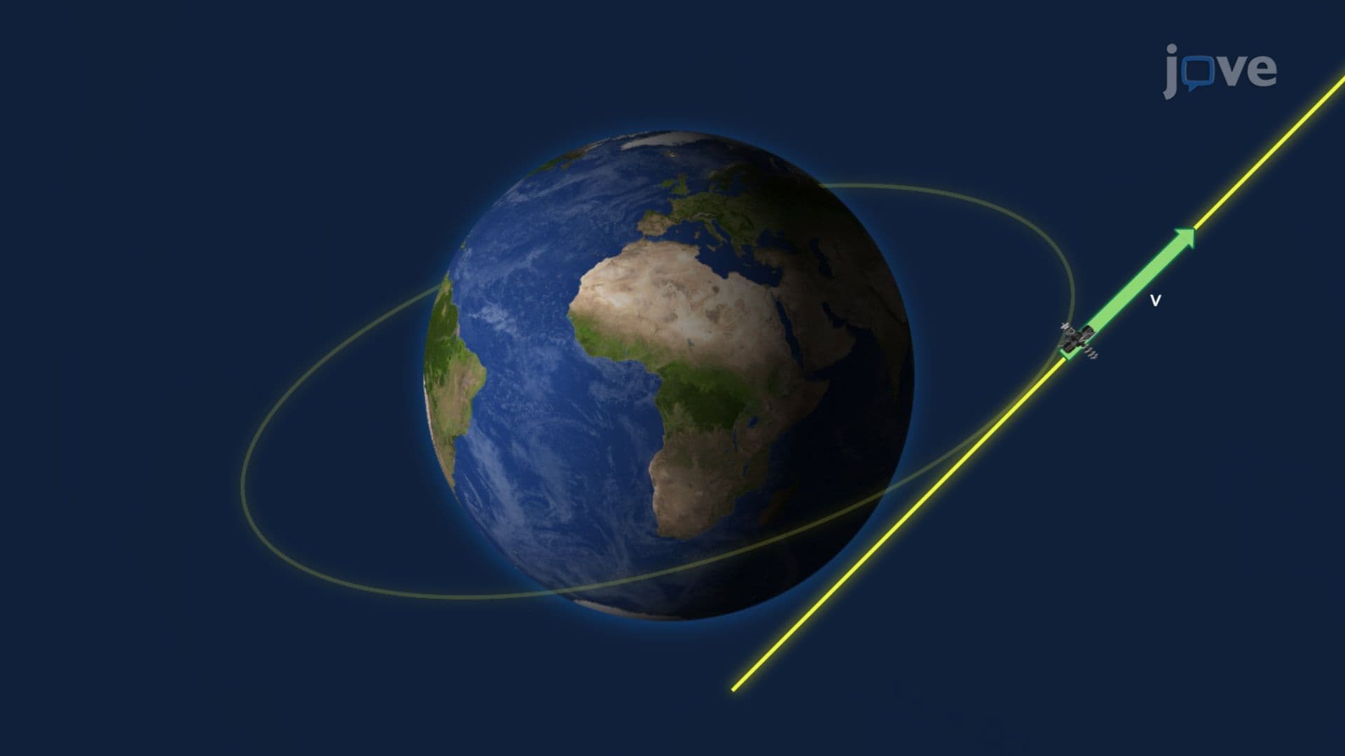
The gradient of a function, written as ∇F, collects all three partial derivatives: ∇F = (∂F/∂x, ∂F/∂y, ∂F/∂z). This vector always points in the direction of steepest increase of F. When a curve r(t) lies entirely on a level surface and passes through a point P, applying the Chain Rule for partial derivatives to the equation F(r(t)) = k yields a dot product: ∇F · r'(t) = 0. Since this equals zero, the gradient is perpendicular to every tangent vector of every curve through P on the surface. That makes ∇F the normal vector to the tangent plane at P, a powerful and elegant result.
Once you have the normal vector ∇F evaluated at point P = (x₀, y₀, z₀), the tangent plane equation follows the standard point-normal plane formula:
∂F/∂x · (x − x₀) + ∂F/∂y · (y − y₀) + ∂F/∂z · (z − z₀) = 0
where each partial derivative is evaluated at P. This formula appears regularly in college Calculus III courses at US universities, as well as in AP Calculus BC extensions and university physics courses covering electromagnetic field surfaces.
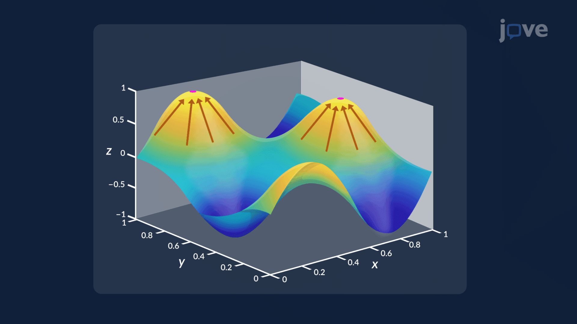
Tangent plane approximations are used in computer graphics to render smooth 3D surfaces in video games and film, studios like Pixar rely on linear approximations to calculate lighting and shading efficiently. In machine learning, gradient vectors on loss surfaces guide optimization algorithms like gradient descent. On college midterms and Calculus III finals across US universities, students are routinely asked to find the equation of a tangent plane to a given level surface at a specified point. Mastering this topic also builds the foundation for studying directional derivatives, maximum and minimum values of functions of two variables, and Lagrange multipliers, all of which depend on a solid understanding of the gradient and its geometric meaning.
Related Micro-courses