Loading video…

 13 Concepts
 47 views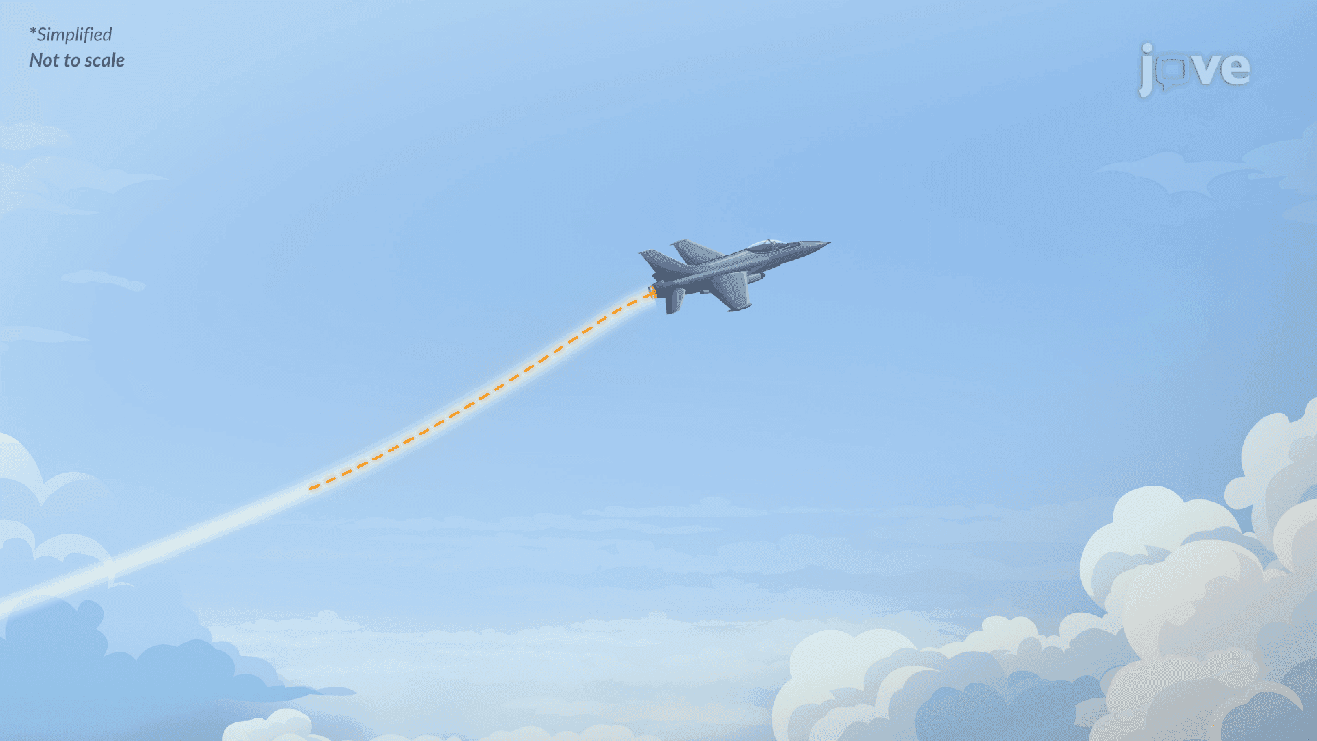

Video Summary: Real World Applications of Space Curves Explained
Did you know radar systems at NORAD must determine in milliseconds whether two objects will collide in three-dimensional space? The real-world applications of space curves make that possible. Real-World Applications of Space Curves Explained shows how vector functions model moving objects as continuous 3D paths, allowing engineers to predict collisions by matching position and time simultaneously across all three coordinate components. Watch the full video on JoVE Coach to master this concept with expert-led visuals and step-by-step explanations.
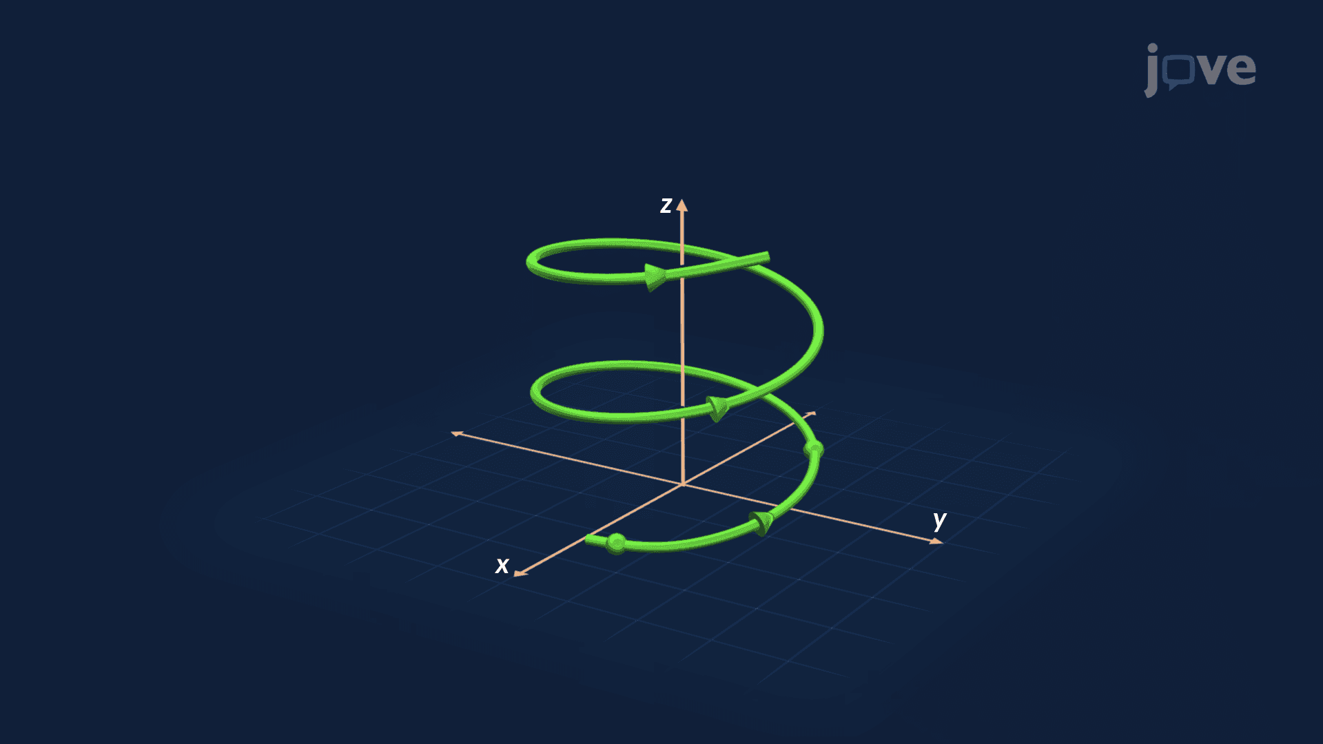
Space curves might sound purely mathematical, but they sit at the foundation of some of the most critical engineering systems in the United States, from missile defense tracking at NORAD to spacecraft trajectory planning at NASA's Jet Propulsion Laboratory. A space curve is simply a path traced in three-dimensional space by a moving point, described mathematically by a vector function r(t) = ⟨x(t), y(t), z(t)⟩. Understanding the real-world applications of space curves means understanding how time-dependent position, velocity, and acceleration all work together to describe motion that no flat, two-dimensional equation can fully capture.
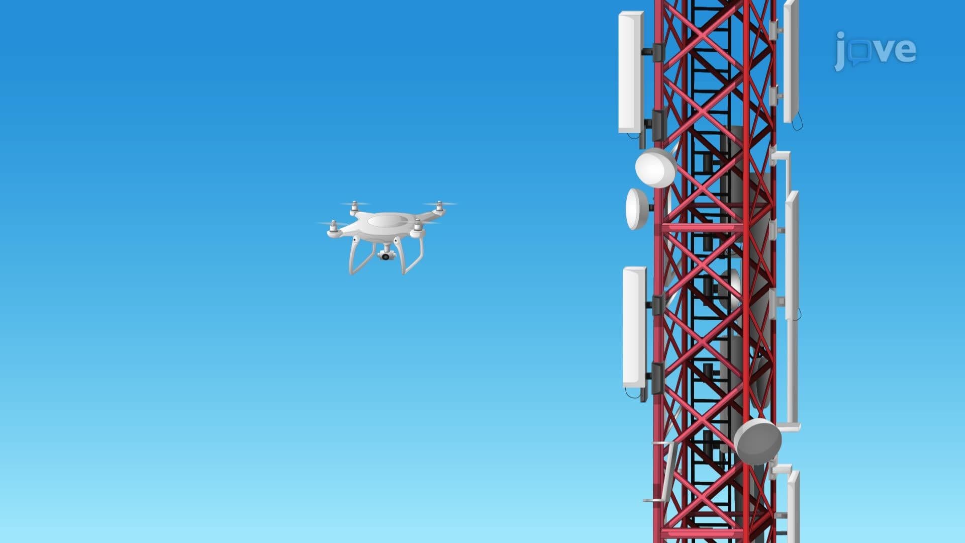
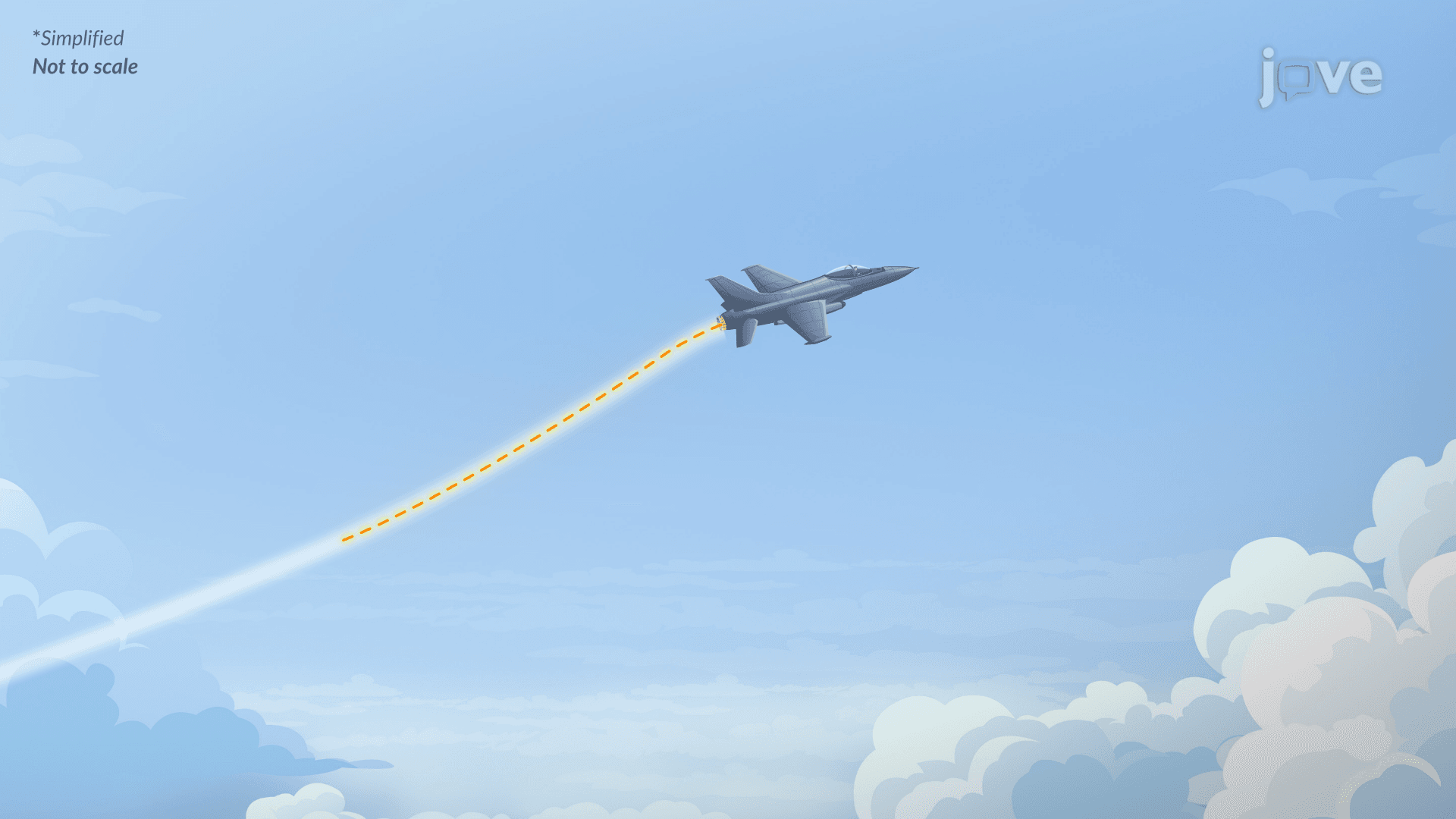
One of the most compelling real-world applications of space curves basics involves collision detection. Imagine two aircraft tracked by a ground-based radar system. Each aircraft follows its own vector function, tracing a unique space curve through the sky. To determine if a collision will occur, engineers set the two position vectors equal, component by component, and solve for time. If a single value of t satisfies all three equations (x, y, and z simultaneously), a collision is imminent. If the objects reach the same point in space at *different* times, the curves intersect geometrically but no collision happens. This subtle but critical distinction is what makes rigorous mathematical modeling essential in aerospace safety.
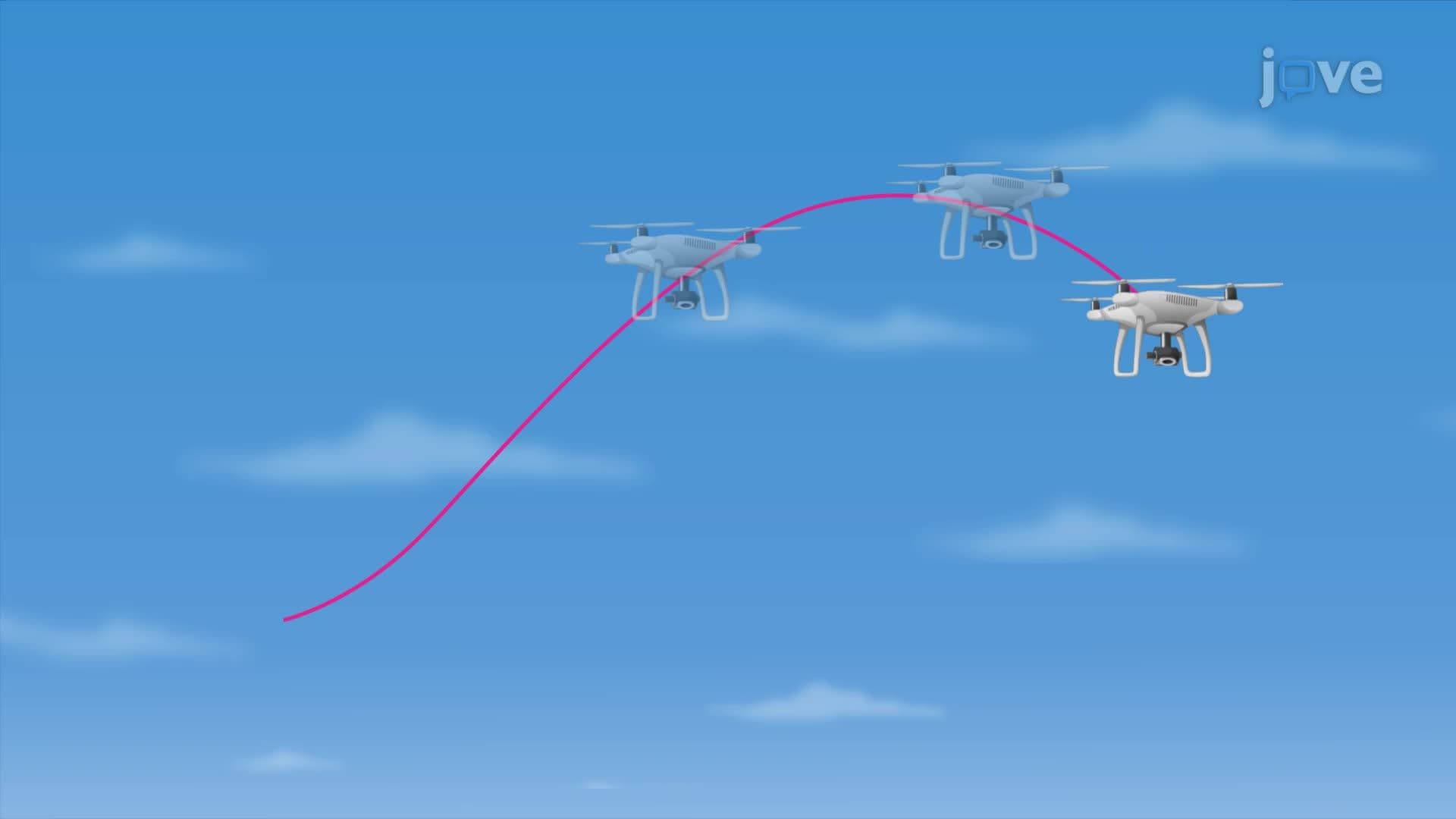
Once a space curve is defined, calculus unlocks deeper physical meaning. The velocity vector is the first derivative of the position vector: v(t) = r'(t). Its direction is always tangent to the curve, giving engineers the unit tangent vector T(t) = r'(t) / |r'(t)|. This tells you *which way* an object is heading at any instant.
Curvature (written as kappa, κ) measures how sharply a path bends at any point. Formally, curvature κ = |T'(t)| / |r'(t)|. A straight-line path has zero curvature; a tight spiral has high curvature. In highway engineering, curvature governs safe speed limits on curved ramps, a direct, everyday application students across the US encounter without realizing it.
The normal vector N(t) points toward the center of curvature, perpendicular to the tangent. The binormal vector B(t) = T(t) × N(t) completes a three-dimensional frame, called the TNB frame, that travels with the moving object and describes its full orientation in space.
The acceleration vector is the second derivative of position: a(t) = r''(t). It splits into two physically meaningful parts: the tangential component (a sub T), which reflects how *fast* speed is changing, and the normal component (a sub N), which reflects how sharply the *direction* is changing. Understanding both components helps explain why a car on a curved highway needs more braking force than one on a straight road, even at the same speed.
The arc length of a space curve from t = a to t = b is computed as the integral of |r'(t)| dt from a to b, a concept tested directly in AP Calculus BC and standard college Calculus III courses at universities like MIT OpenCourseWare-aligned programs across the country.
For AP Calculus BC students, space curves and parametric motion appear in free-response questions. For college undergraduates in Calculus III or Multivariable Calculus, midterms and finals routinely ask students to find curvature, arc length, and the TNB frame. Mastering these concepts with concrete real-world context, not just formulas, is the key to high-stakes exam success.
Related Micro-courses