Loading video…

 13 Concepts
 47 views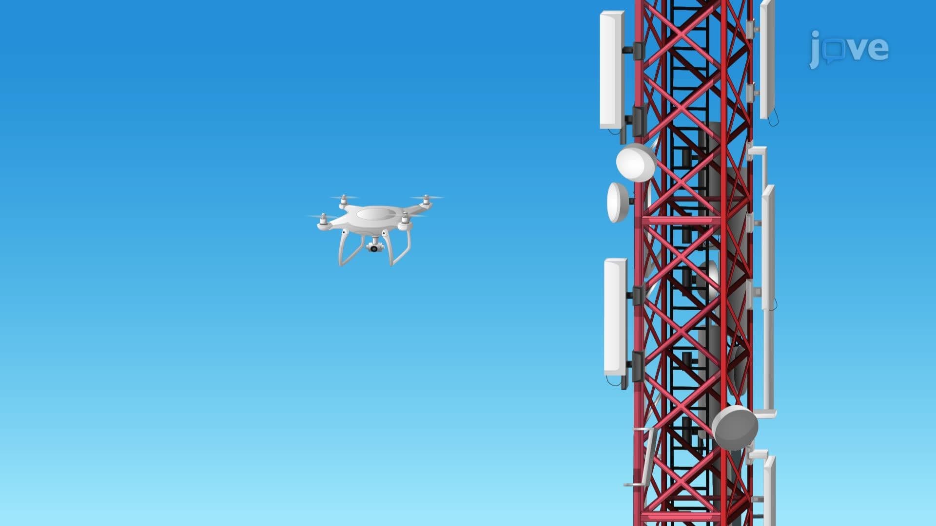

Video Summary: Problem Solving in Vector Functions and Motion
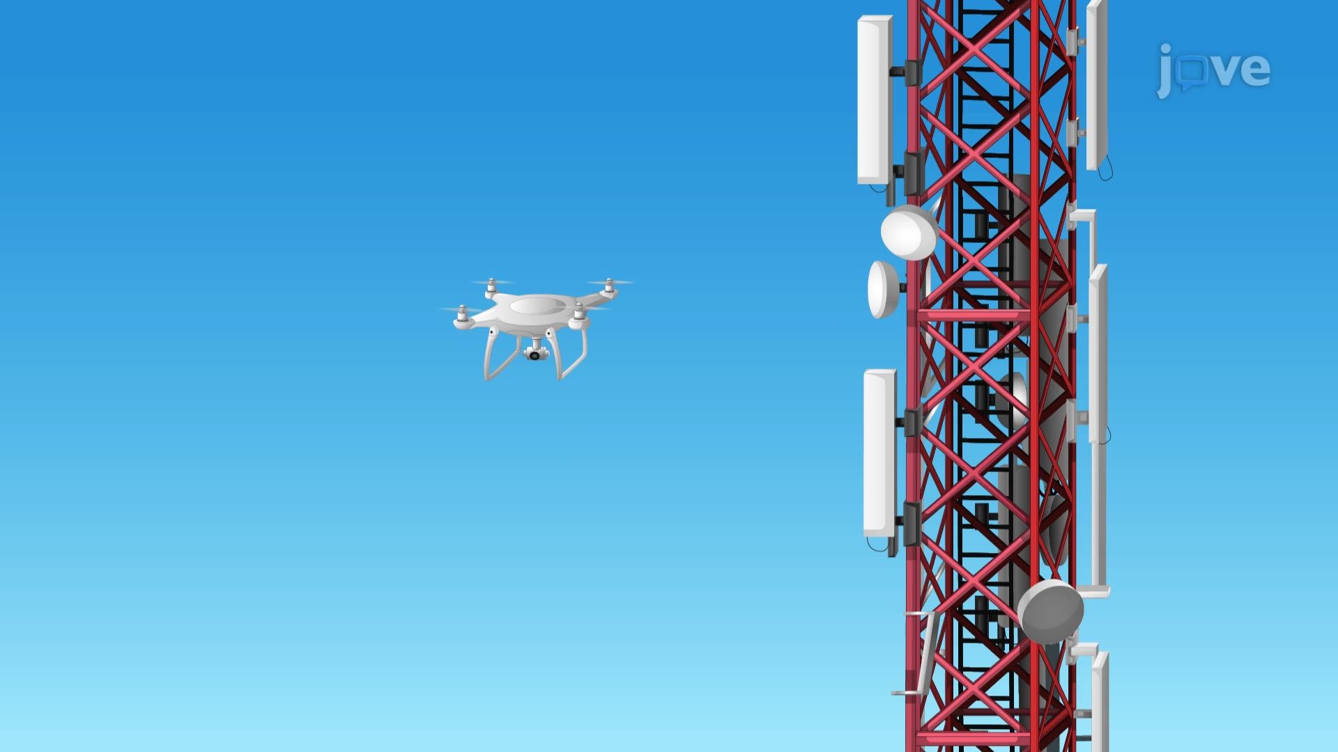
Did you know engineers tracking a drone inspecting a skyscraper use the same calculus you learn in class? Problem solving in vector functions and motion is the mathematical backbone behind autonomous flight path planning. Master the problem solving in vector functions and motion basics, integrating acceleration to find velocity, then integrating again for position, and you unlock real-world tools used by aerospace engineers across the US. Watch the full video on JoVE Coach to master this concept with expert-led visuals and step-by-step explanations.
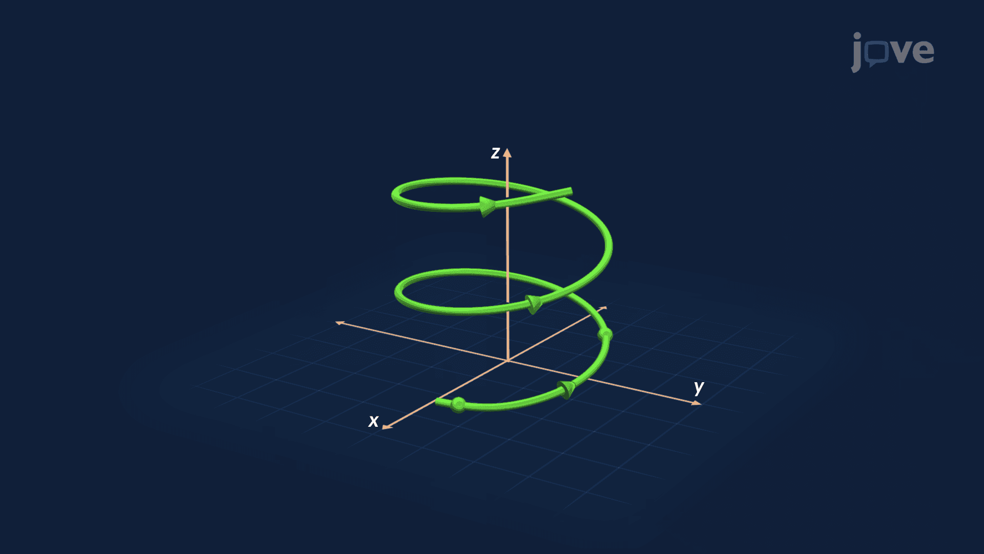
When a NASA drone surveys a launch tower at Kennedy Space Center, it doesn't just move forward, it curves, rises, and adjusts direction simultaneously. That three-dimensional motion is described entirely by vector functions. Problem solving in vector functions and motion means using calculus, specifically integration and differentiation, to translate physical laws like Newton's second law into precise mathematical paths. This concept appears in AP Calculus BC, college Calculus III, and introductory physics and engineering courses nationwide.
The core technique works in two steps. First, integrate the acceleration vector a(t) with respect to time to produce the velocity vector v(t). The constant of integration is not just a number, it's a vector, determined by substituting the known initial velocity at t = 0. Second, integrate v(t) to find the position vector r(t), again solving for the vector constant using the object's starting position. Each step mirrors single-variable calculus, but every component, x, y, and z, is handled simultaneously. AP Calculus BC exams frequently test this two-step integration chain with initial conditions, making it a high-priority skill for exam preparation.
Once you have r(t), a rich geometric description opens up. The unit tangent vector T(t) points in the direction of motion at each instant, found by normalizing r'(t). The normal vector N(t) points toward the center of curvature, it tells you which way the path is bending. Together with the binormal vector B(t) = T × N, these three vectors form the Frenet-Serret frame, a moving coordinate system attached to the object. Curvature (κ) measures how sharply the path bends at any point; a straight road has κ = 0, while a tight curve on a NASCAR oval has high κ. The arc length of a space curve is computed by integrating the magnitude of r'(t), giving total distance traveled regardless of direction changes. College Calculus III midterms commonly ask students to compute these quantities from a given parametric path.
A powerful application is decomposing acceleration into two physically meaningful parts. The tangential component (a_T) measures how fast the object is speeding up or slowing down along the path. The normal component (a_N) measures how sharply the object is turning, it depends directly on curvature and speed. For a SpaceX rocket performing a pitch maneuver, the tangential component reflects engine thrust changing speed, while the normal component reflects the guidance system steering the vehicle. Understanding how to find the acceleration vector from position, by differentiating twice, and then decomposing it this way is a skill tested in both university physics finals and engineering dynamics courses across the US.
Related Micro-courses