Loading video…


 14 Concepts
 4.7K views

Video Summary: What Is Simpson S Rule I
How do land surveyors calculate the area of an irregular plot bordered by a winding river? Simpson's Rule I offers a powerful solution. This numerical integration technique estimates areas under curved boundaries using just a few equally spaced measurements, no complex river equation needed. US civil engineers routinely apply this method in land surveys and infrastructure planning. Watch the full video on JoVE Coach to master this concept with expert-led visuals and step-by-step explanations.
Simpson's Rule I is a foundational numerical integration method used to approximate the area under a curve when an exact mathematical formula for that curve is unavailable or impractical. Rather than requiring a precise equation, it works from a small number of measured data points, making it indispensable in fields like civil engineering, environmental science, and applied mathematics. Understanding this method also deepens your grasp of core calculus concepts tested in AP Calculus AB/BC and college-level courses.
The key insight behind Simpson's Rule I is elegant: instead of approximating a curve with flat rectangles (as in Riemann sums) or straight-line trapezoids, it fits a parabola through three equally spaced points. A parabola is a quadratic curve, smooth and curved, which far more accurately mirrors the shape of natural boundaries like riverbanks, coastlines, or irregular terrain.
Those three points correspond to perpendicular measurements taken at equal spacing h apart. Label them y0 (left), y1 (center), and y2 (right). The unique parabola passing through all three is then integrated over the interval, yielding the famous formula:
Area ≈ (h/3)(y0 + 4y1 + y2)
Notice that the center measurement y1 carries a weight of 4, while the outer measurements each carry a weight of 1. This weighting reflects the parabola's shape, the middle of the curve contributes more to the total area.
To derive this formula, the parabola is expressed as a general quadratic: y = A·x² + B·x + C, centered so that the middle point sits at x = 0. This centering simplifies the algebra considerably. Because y1 is at x = 0, the constant C equals y1 directly. Substituting the outer points (at x = −h and x = +h) into the equation and solving gives expressions for A and B in terms of y0, y1, and y2. Integrating the quadratic over the interval from −h to +h and substituting these values produces the final formula. This derivation process exercises skills directly relevant to AP Calculus BC topics including polynomial integration and applying limits.
American civil engineers use Simpson's Rule I when surveying irregularly shaped land parcels, particularly in river floodplain mapping, highway right-of-way calculations, and environmental impact assessments. The US Army Corps of Engineers, for example, applies numerical integration techniques routinely when modeling flood zones along major rivers like the Mississippi or Missouri.
In academic settings, Simpson's Rule I appears in AP Calculus BC curriculum under numerical methods, and is a common topic in college calculus courses (Calc II) nationwide. Students may encounter it alongside related techniques such as integration by parts, trigonometric substitution, partial fractions, and trigonometric integrals, all methods for handling integrals that resist straightforward antiderivative computation. Understanding how to choose an integration technique is itself a critical skill: Simpson's Rule I is the go-to choice when the function is unknown or defined only by data points.
Simpson's Rule I sits at the intersection of practical measurement and theoretical calculus. It bridges the gap between improper integrals (where standard techniques may fail) and applied problem-solving. Students who master this method gain an intuitive understanding of why quadratic approximations are more powerful than linear ones, a concept that resurfaces in Taylor series, error analysis, and numerical methods courses at the undergraduate level. Whether you're preparing for a college midterm or building skills for engineering coursework, Simpson's Rule I is a concept worth understanding deeply.
Related Micro-courses