Loading video…

 6 Concepts
 2.5K views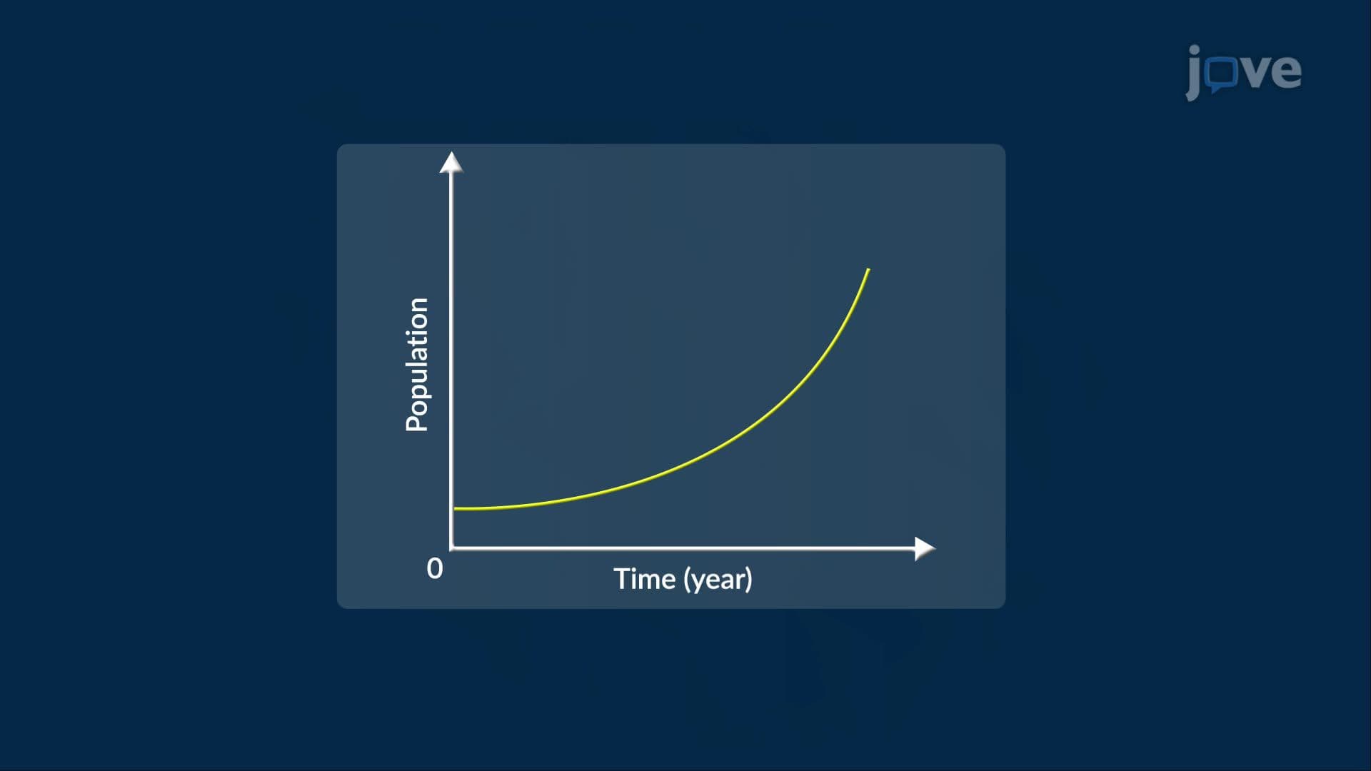

Video Summary: Differential Equations Modeling
Why do some populations explode while others stabilize? Differential equations modeling answers exactly that, and it's more powerful than most students realize. From predicting US national park wildlife counts to forecasting campus enrollment, this framework turns real-world assumptions into solvable equations. The logistic growth model, a cornerstone of differential equations modeling, captures how limited resources shape population limits. Watch the full video on JoVE Coach to master this concept with expert-led visuals and step-by-step explanations.
Differential equations modeling is the process of using differential equations to represent how a quantity changes over time or space based on a set of logical assumptions. Rather than describing *where* something is, these equations describe *how fast* it's changing, and why. This makes them one of the most powerful tools in mathematics, science, and engineering. In a standard college calculus or differential equations course, students first encounter this idea through population growth, where the math stays accessible but the conceptual depth is enormous.
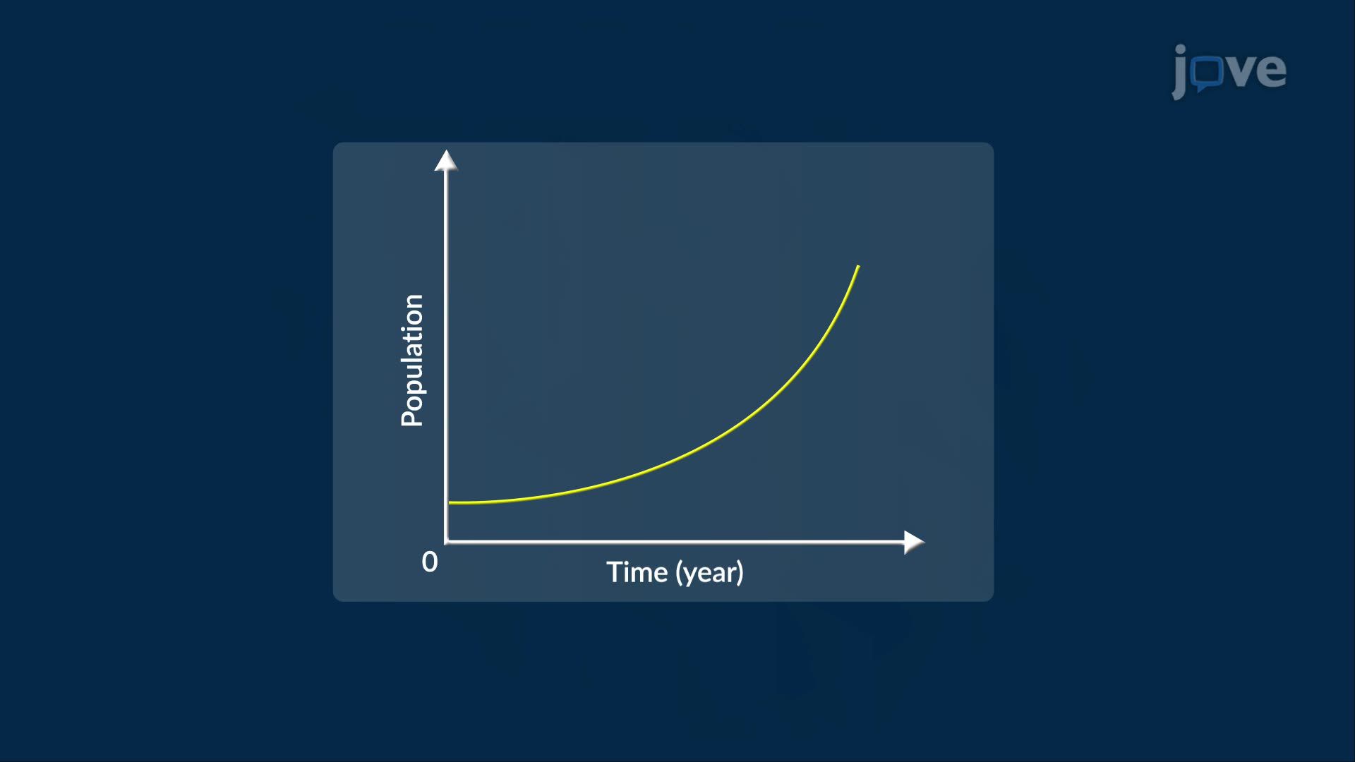
Every model starts with assumptions. The simplest population model assumes unlimited resources, meaning every individual contributes equally to growth regardless of how crowded the environment is. Mathematically, this means the rate of change of population P with respect to time t is proportional to P itself: dP/dt = kP, where k is a positive growth constant. This is a first-order linear ordinary differential equation, and its solution is the classic exponential function P(t) = P(0) · e^(kt). While elegant, this model breaks down quickly in real settings, no environment has truly unlimited resources.
The logistic growth model corrects the exponential model by adding a second assumption: growth slows as the population approaches a maximum sustainable size, called the carrying capacity M. When P is much smaller than M, the model behaves nearly like exponential growth. When P approaches or exceeds M, a corrective term kicks in that reduces or reverses growth. The resulting equation is dP/dt = kP(M − P), a separable differential equation. Solving it requires separating variables and applying partial fractions, skills directly tested in AP Calculus BC and first-semester college differential equations courses. The solution produces an S-shaped (sigmoidal) curve, one of the most recognizable patterns in biology and ecology.
This framework isn't just academic. The US Fish and Wildlife Service uses logistic-style models to manage deer and elk populations in national parks. Epidemiologists at the CDC apply similar equations to model the spread of infectious diseases, where the "carrying capacity" is the susceptible population. In AP Calculus BC, students are directly tested on setting up and solving separable differential equations, interpreting slope fields, and connecting solutions to initial value problems. On college midterms in courses like Math 246 or Engineering Differential Equations, logistic growth problems regularly appear because they test multiple skills at once: model interpretation, algebraic manipulation, and solution analysis. Understanding the conceptual story behind the equation, not just the procedure, is what separates strong exam performance from memorization.
Two solution strategies are essential for this topic. First, separation of variables applies when you can rewrite dP/dt so that all P terms are on one side and all t terms are on the other, then integrate both sides independently. Second, integrating factors are used for linear first-order equations that can't be separated directly. In both cases, a general solution contains an arbitrary constant C, while a particular solution uses a given initial condition, like P(0) = 500 deer, to solve for C exactly. Mastering these techniques gives students the foundation to tackle any first-order differential equation they'll encounter in science, engineering, or economics coursework.
Related Micro-courses