Loading video…

 6 Concepts
 2.5K views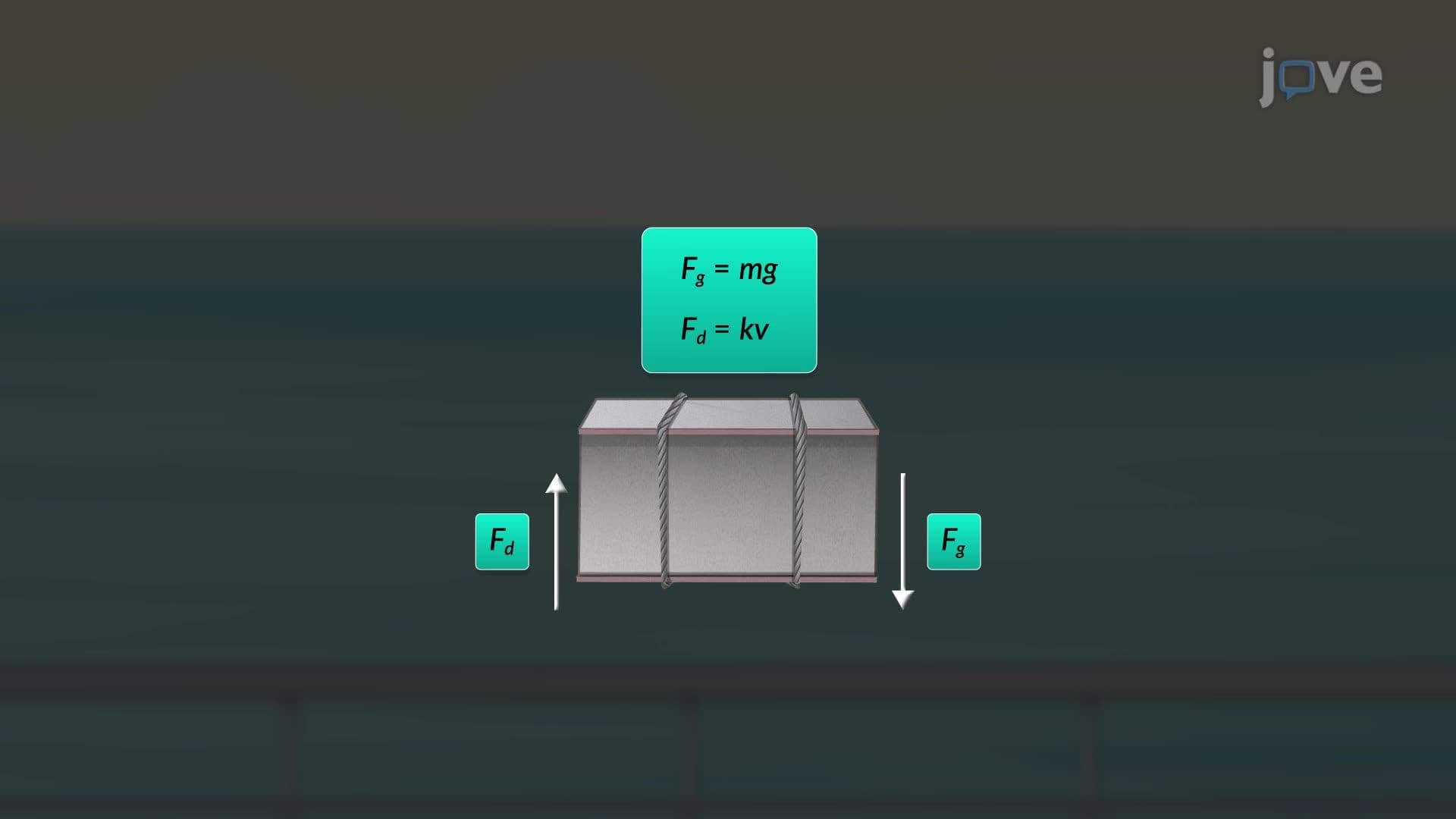

Video Summary: Problem Solving in Differential Equations
Did you know a falling object never accelerates forever, physics puts a natural speed limit on it? Problem solving in differential equations reveals exactly why, using real forces like gravity and air resistance. Engineers at US shipyards use similar drag-force models to test equipment safety under realistic conditions. Problem Solving in Differential Equations transforms these physical scenarios into solvable mathematical models. Watch the full video on JoVE Coach to master this concept with expert-led visuals and step-by-step explanations.
A differential equation is any equation that relates a function to its own rate of change. Problem solving in differential equations is the structured process of setting up, simplifying, and solving these equations to describe real phenomena, from a ship's test weight falling through air to a parachutist's descent over the Rocky Mountains. The skill is central to AP Calculus BC, college-level Calculus II, and introductory physics and engineering courses across US universities.
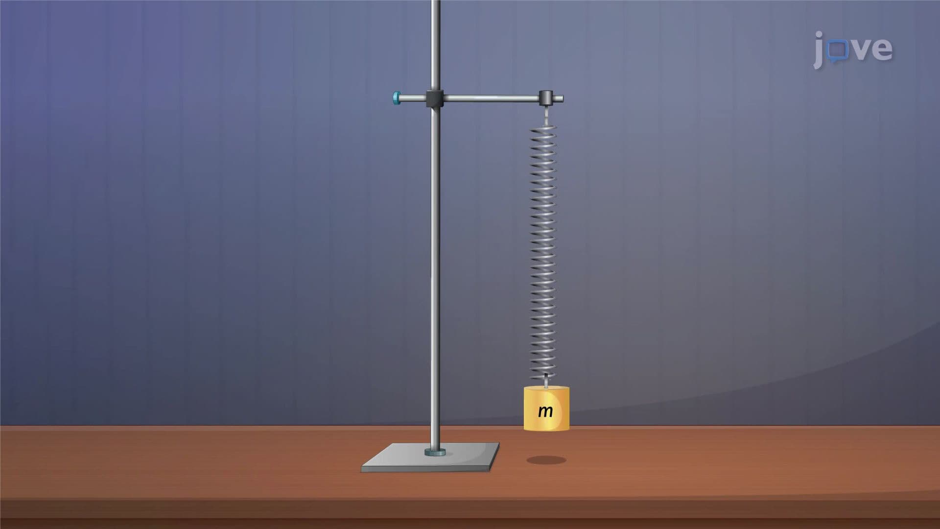
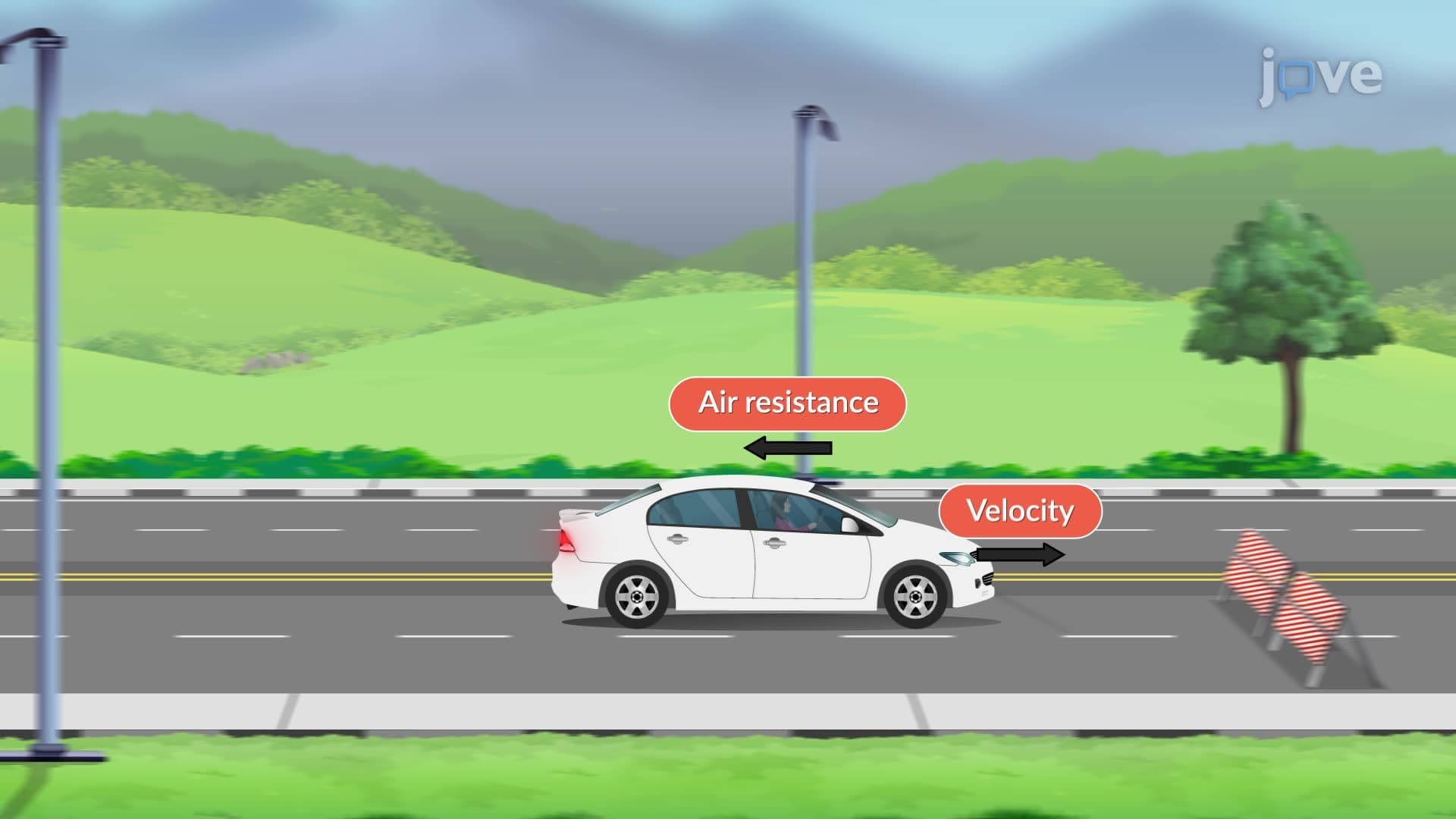
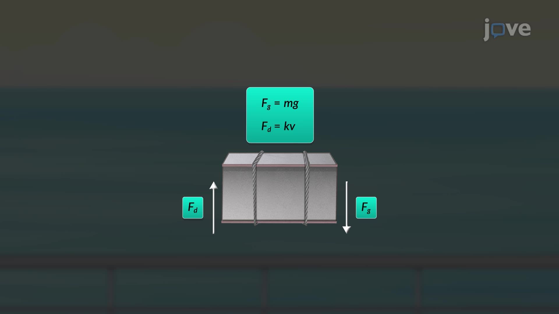
Every problem-solving process starts with a physical law. Here, Newton's Second Law states that the net force acting on an object equals mass times acceleration: F(net) = m * a. Since acceleration is the derivative of velocity with respect to time, this becomes a differential equation. For a falling object, two forces act simultaneously: gravity pulling downward (F = m * g) and aerodynamic drag pushing upward (F(drag) = k * v, where k is the drag constant and v is velocity). The net force equation becomes:
m * (dv/dt) = m * g - k * v
Dividing both sides by mass simplifies the equation and introduces the parameter b = k/m, giving:
dv/dt = g - b * v
This is a linear first-order ordinary differential equation, one of the most commonly tested equation types in US calculus and physics curricula.
The equation dv/dt = g - b*v is separable, meaning all terms involving v can be moved to one side and all terms involving t to the other. Rearranging gives:
dv / (g - b*v) = dt
Integrating both sides yields a natural logarithm on the left and t plus a constant on the right. Solving for v produces an exponential equation of the form:
v(t) = (g/b) + C * e^(-b*t)
This is the general solution. The constant C is determined by applying the initial condition. Since the weight starts from rest, v(0) = 0, which means C = -(g/b). Substituting back gives the particular solution:
v(t) = (g/b) * (1 - e^(-b*t))
This type of initial value problem, where a starting condition pins down the unique solution, appears regularly on AP Calculus BC free-response questions and college midterms nationwide.
As time increases, the term e^(-b*t) approaches zero, so velocity approaches a constant value: v(terminal) = g/b. This is terminal velocity, the maximum speed a falling object reaches when drag exactly balances gravity. For a 10-kilogram weight with a drag constant of 2 newton-seconds per meter, the model predicts:
v(terminal) = (9.8 * 10) / 2 = 49 meters per second
This result has direct engineering relevance. Aerospace engineers at companies like Boeing and NASA model drag forces on descending payloads using identical mathematical frameworks. Sports scientists study terminal velocity in skydiving to design safer equipment. Understanding this long-term behavior, reading the exponential solution and knowing it stabilizes, is a critical analytical skill tested in both AP Physics C: Mechanics and university-level differential equations courses.
The four-step framework, identify forces, write the differential equation, separate and integrate, apply initial conditions, is universally transferable. It applies to RC circuit analysis in electrical engineering, population growth models in AP Environmental Science, and drug concentration decay models in pre-med pharmacology courses. Mastering this workflow in a clear physical context like falling-body motion gives students a reusable template they can adapt to any first-order separable or linear equation they encounter.
Related Micro-courses