Loading subject page…

- Physics
- Motion Along a Straight Line
- Kinematic Equations - II
Micro-course: Motion Along a Straight Line
224,217 views
Learn key concepts and earn your certificate.


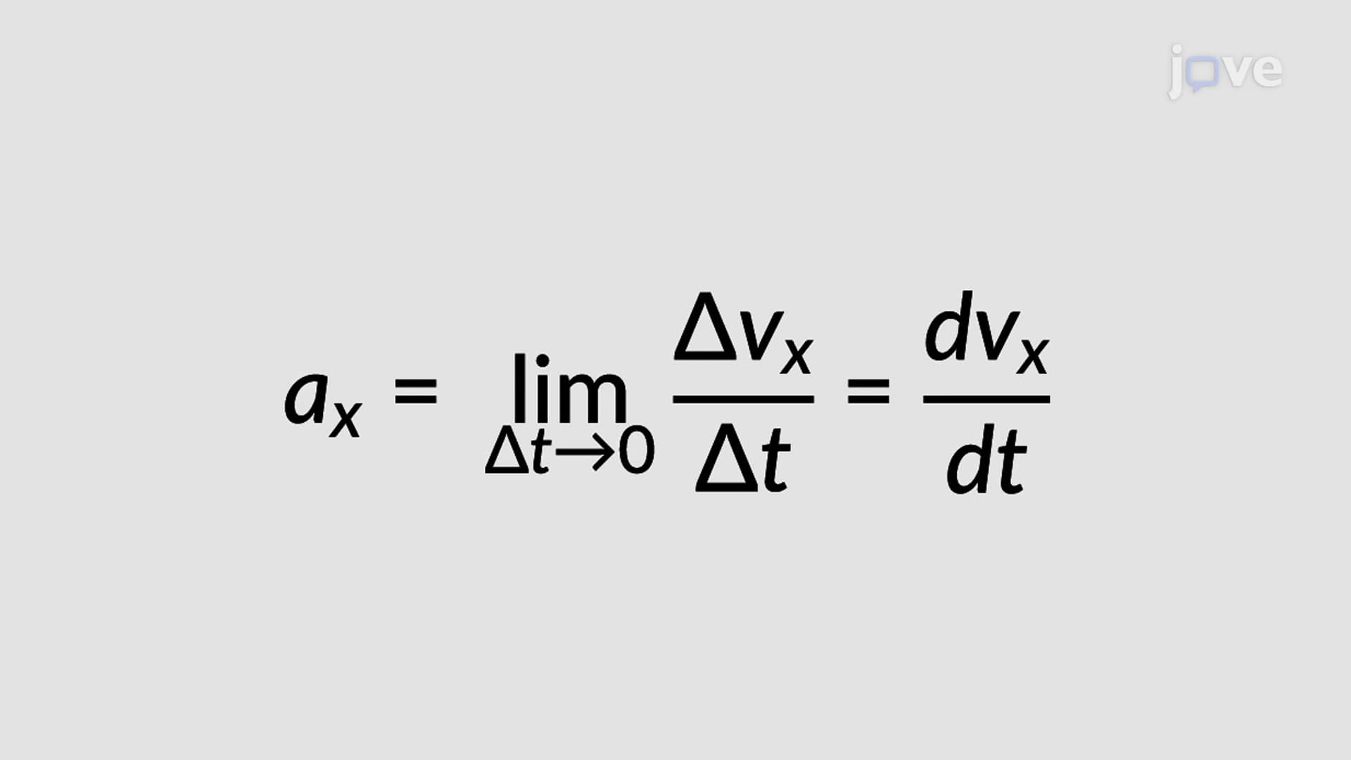
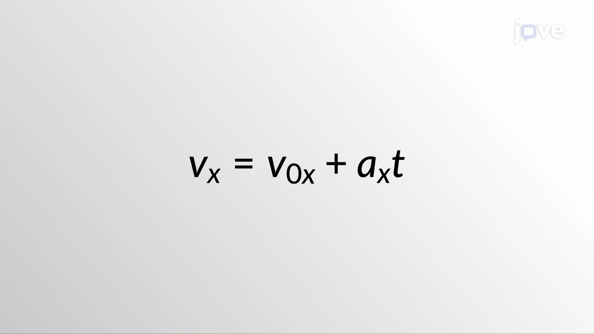
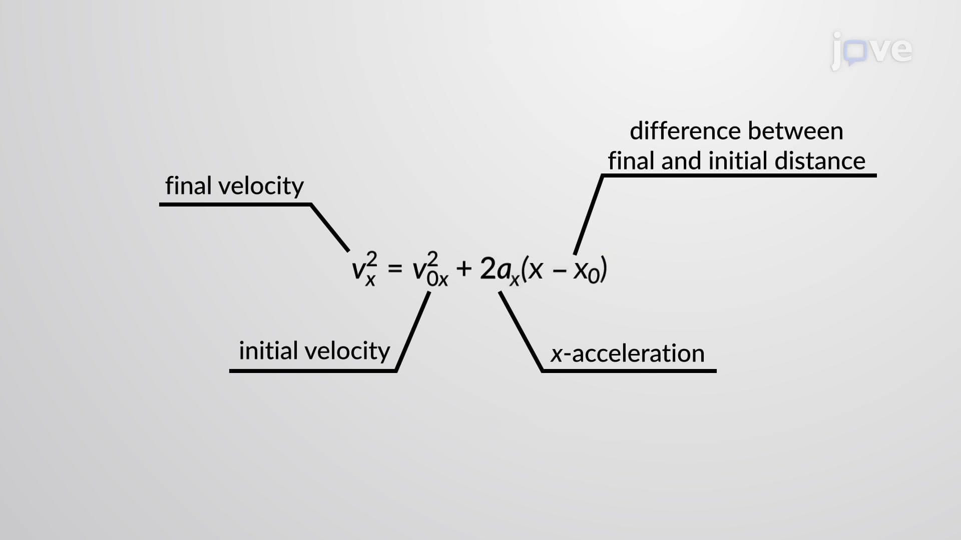
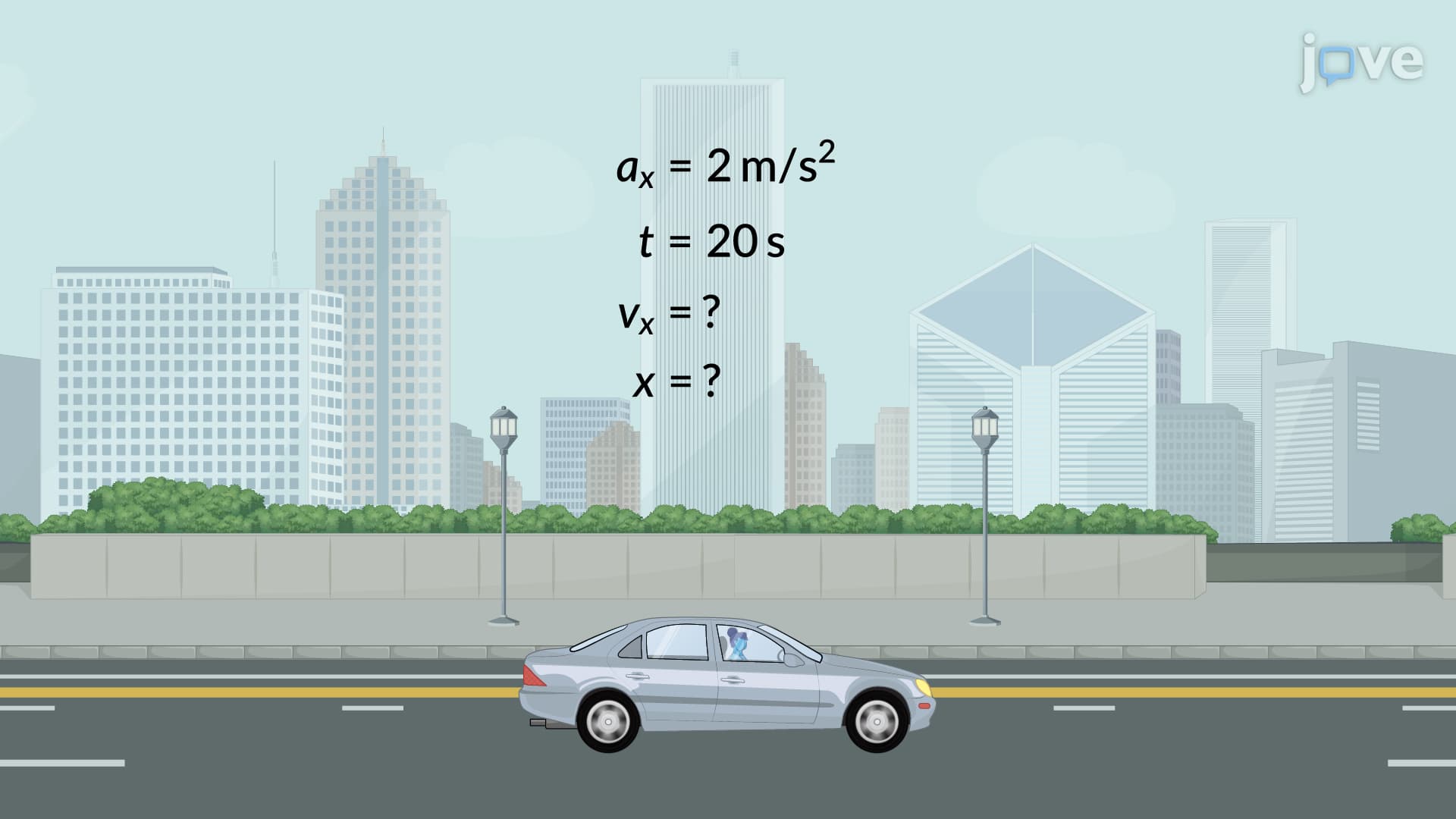


Kinematic Equations - II

00:00
01:17
Video Summary: What Is Kinematic Equations Ii
Ever wonder how NASA calculates the precise trajectory for a Mars rover landing? Kinematic equations II forms the mathematical foundation for predicting an object's position at any given moment during motion with constant acceleration. This second kinematic equation builds upon velocity concepts to determine where a baseball will land after leaving a pitcher's hand or how far a car travels during braking. Understanding What is Kinematic Equations II unlocks the ability to solve complex motion problems in physics and engineering applications. Watch the full video on JoVE Coach to master this concept with expert-led visuals and step-by-step explanations.
- Understand What is Kinematic Equations II and how it relates position, initial velocity, acceleration, and time in a single mathematical relationship
- Identify the key components of the second kinematic equation: initial position, constant velocity displacement, and accelerated motion displacement
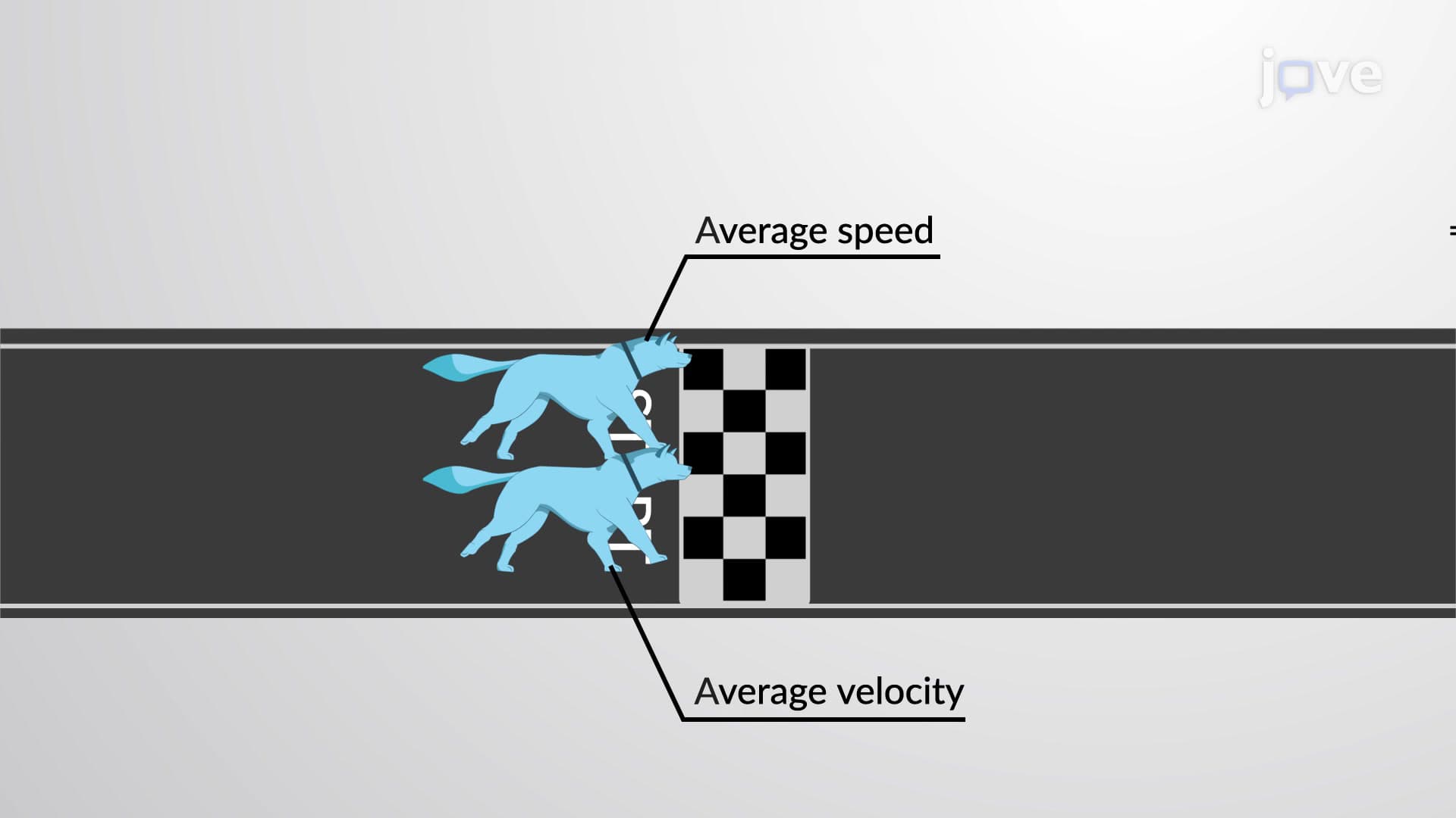
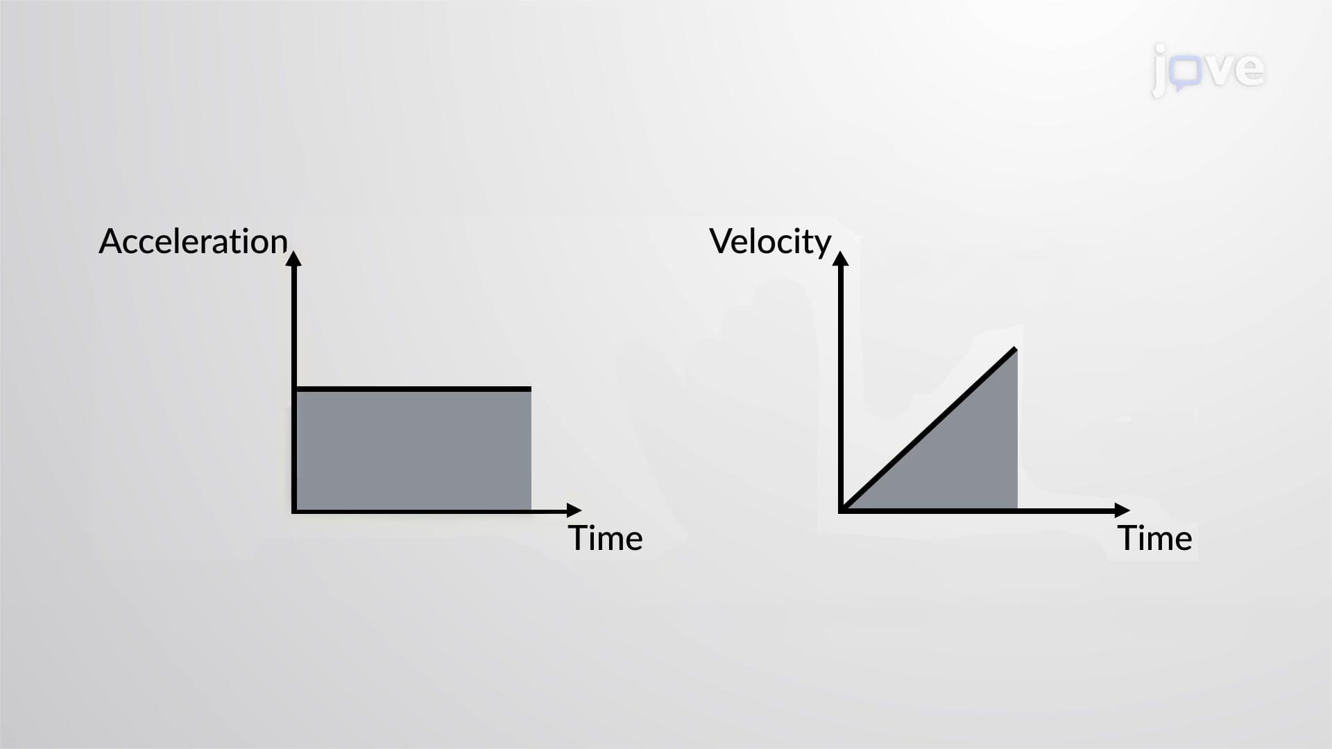
- Analyze how average velocity can be calculated using two different approaches: displacement over time and the mean of initial and final velocities
- Apply the second kinematic equation to solve real-world motion problems involving cars, projectiles, and falling objects
- Recognize the physical meaning behind each term in the position equation and how they contribute to total displacement
- Evaluate when to use kinematic equations II versus other motion equations based on given variables and unknowns
- Compare the mathematical derivation process using average velocity concepts with practical problem-solving applications
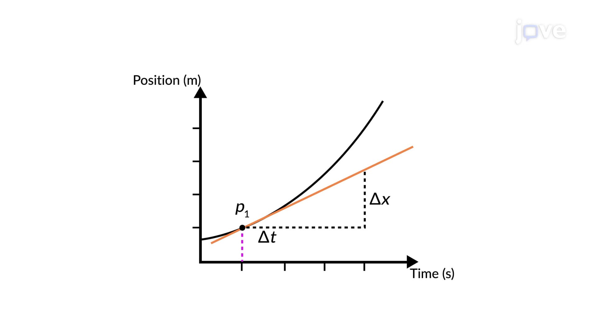
- Explore the connection between kinematic equations II and graphical representations of motion on position-time graphs
Understanding Kinematic Equations II Fundamentals
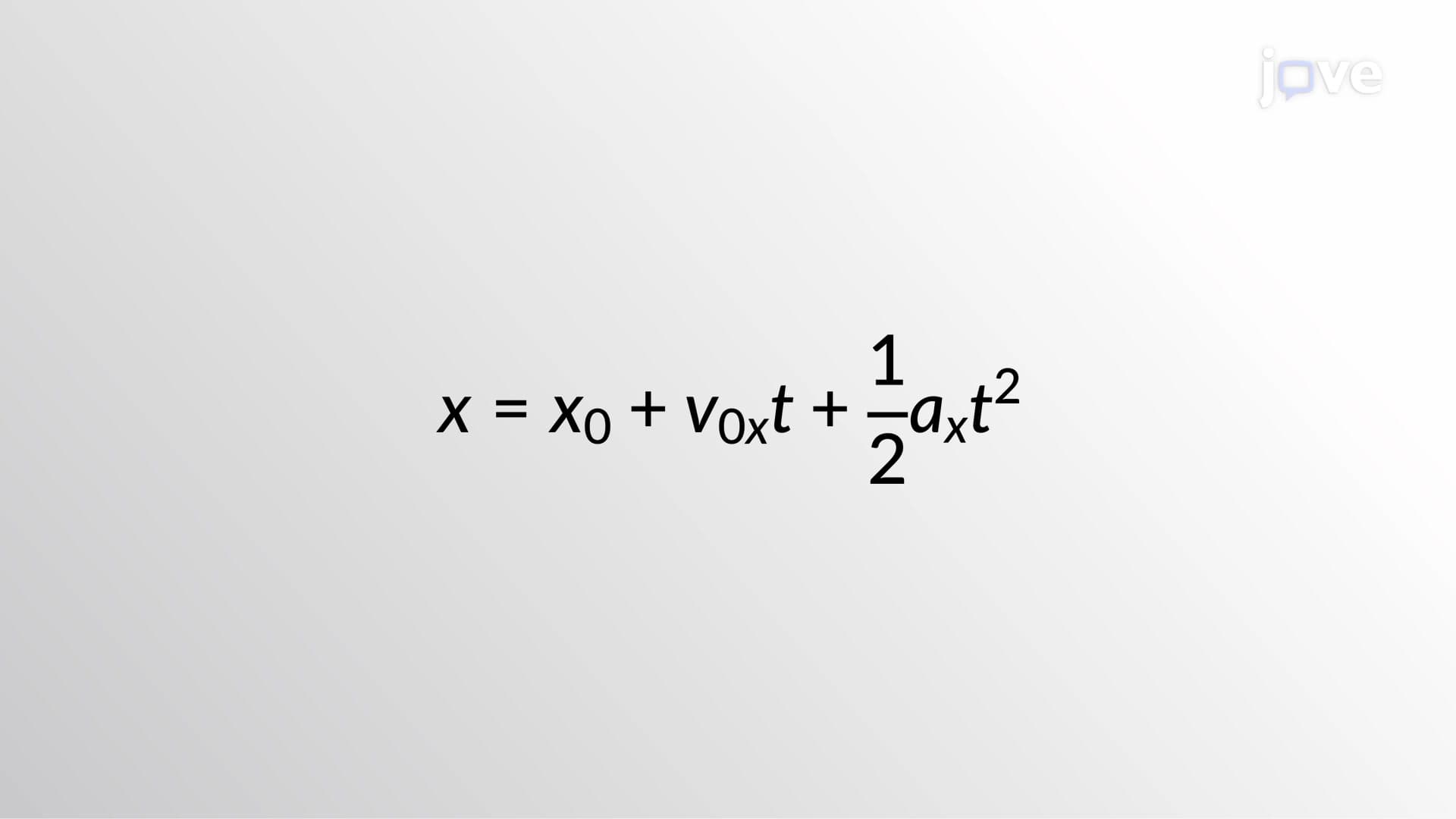
Kinematic equations II represents the second of four essential equations describing motion with constant acceleration. While the first kinematic equation focuses on velocity changes over time, the second equation addresses a fundamental question: where will an object be at a specific moment? This equation, expressed as x = x₀ + v₀t + ½at², combines three distinct contributions to an object's final position.
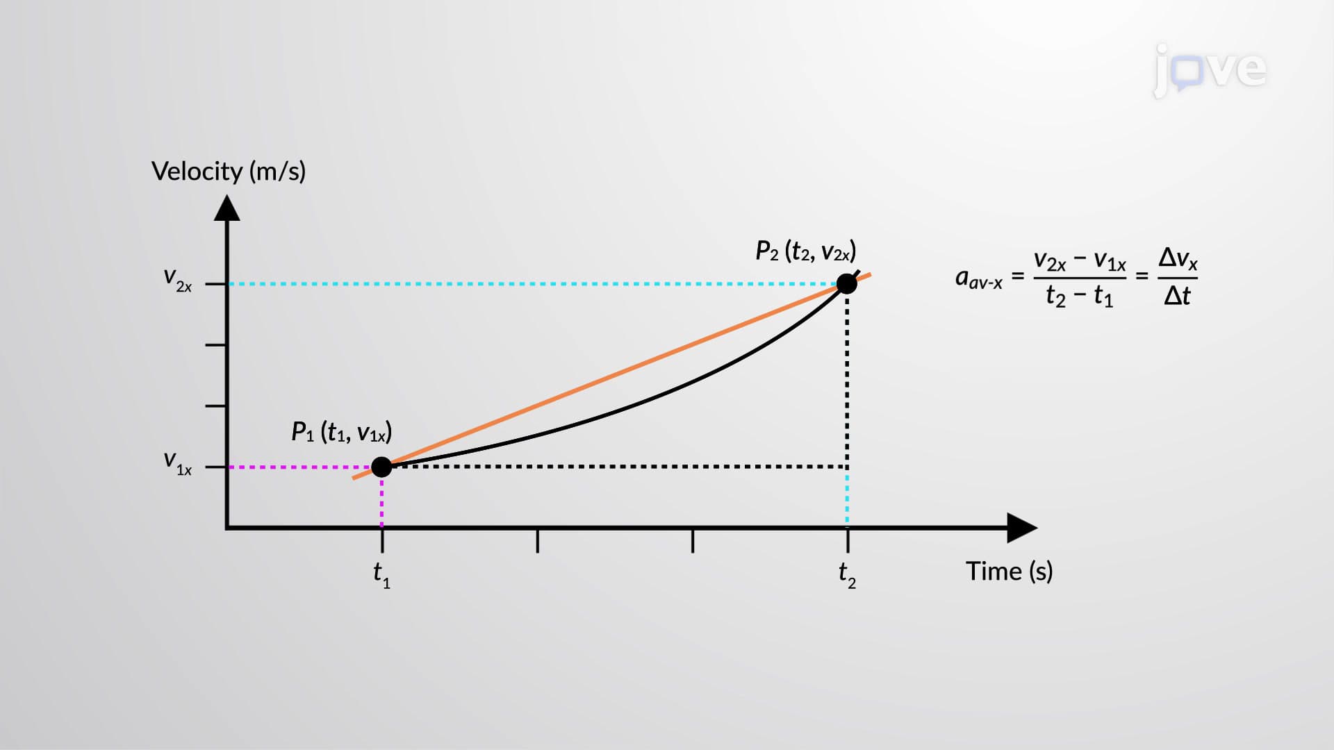
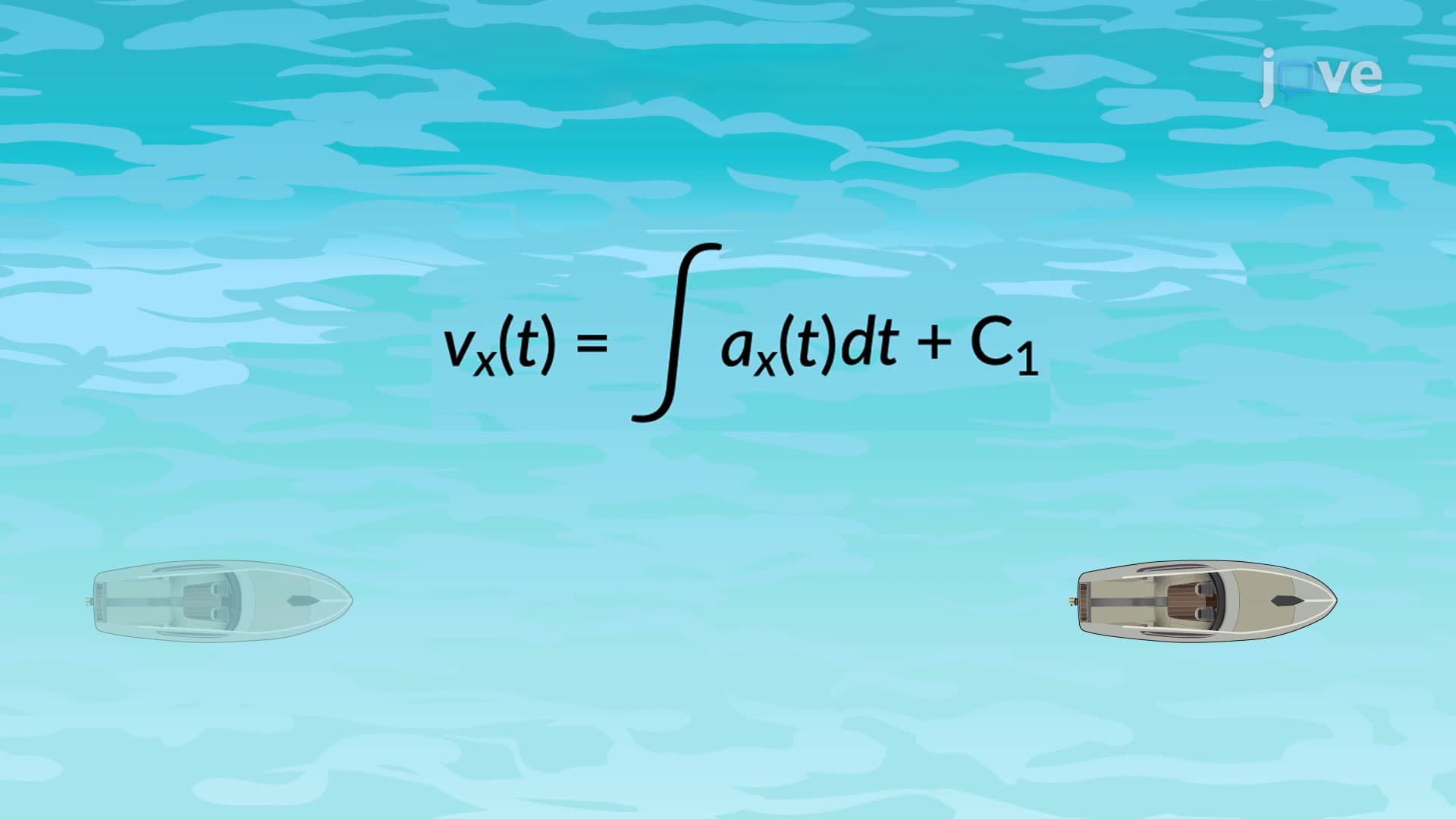
The derivation begins with two equivalent expressions for average velocity. The first definition uses the familiar relationship of displacement divided by time interval. The second approach recognizes that under constant acceleration, average velocity equals the arithmetic mean of initial and final velocities. By setting these equal and substituting the first kinematic equation, we arrive at the position equation.
Breaking Down the Position Equation Components
Each term in kinematic equations II has clear physical significance. The initial position (x₀) establishes the starting reference point. The term v₀t represents distance covered if the object maintained constant initial velocity throughout the entire time interval. Finally, ½at² accounts for additional displacement due to acceleration, whether speeding up or slowing down.
Consider a Tesla Model S accelerating from rest at a traffic light. If the car accelerates at 3.0 m/s² for 5 seconds, starting from position zero, the final position becomes: x = 0 + 0(5) + ½(3.0)(5)² = 37.5 meters. The ½at² term dominates since initial velocity was zero.
Real-World Applications and Problem-Solving Strategies
Understanding kinematic equations II proves crucial for AP Physics students and college freshmen tackling mechanics problems. The equation appears frequently on standardized tests like the AP Physics 1 exam, where students must analyze projectile motion, vehicle dynamics, or falling object scenarios.
For example, calculating how far a football travels horizontally during its flight requires breaking motion into components and applying kinematic equations II to each direction. Similarly, automotive safety engineers use these principles to determine stopping distances for different vehicle speeds and road conditions.
Exam Preparation and Common Applications
Students preparing for physics exams should master identifying which kinematic equation to use based on given information. Kinematic equations II works best when you know initial position, initial velocity, acceleration, and time, but need to find final position. Practice problems often involve objects dropped from buildings, cars accelerating or braking, or projectiles launched at various angles, all common scenarios in American high school and college physics curricula.
Frequently Asked Questions
Kinematic equations II is the mathematical relationship x = x₀ + v₀t + ½at² that predicts an object's position at any time during constant acceleration. It's essential because it connects an object's starting conditions with its future location, making it indispensable for solving motion problems in physics courses, engineering applications, and real-world scenarios like vehicle safety analysis and sports trajectory calculations.
The AP Physics 1 exam frequently tests kinematic equations II through projectile motion, inclined plane, and free-fall problems. Students must identify when to use this equation based on given variables, manipulate the formula to solve for unknowns, and interpret results in physical contexts. Practice with multi-step problems involving both horizontal and vertical motion components is crucial for exam success.
The first kinematic equation (v = v₀ + at) describes how velocity changes over time, while kinematic equations II (x = x₀ + v₀t + ½at²) predicts position changes over time. The first equation helps find final velocity or acceleration, whereas the second determines where an object will be located. Both equations work together to provide complete motion descriptions under constant acceleration.
Use kinematic equations II when you know three of these four variables: initial position (x₀), initial velocity (v₀), acceleration (a), and time (t), and need to find final position (x). If you need final velocity instead, use the first kinematic equation. For problems without time information, consider the third or fourth kinematic equations that relate velocity, acceleration, and displacement directly.
NASA's Mars rover landings demonstrate kinematic equations II perfectly. Engineers calculate the rover's position during atmospheric entry by considering its initial altitude, entry velocity, and deceleration due to atmospheric drag and parachute deployment. This precise positioning ensures the rover lands within the target zone, showcasing how kinematic equations II enables complex space mission success.
Kinematic equations II is very manageable for high school students with basic algebra skills. The equation involves straightforward mathematical operations: addition, multiplication, and squaring. Most students find it easier than solving systems of equations or working with logarithms. Focus on understanding what each term represents physically rather than memorizing the formula, and practice with familiar scenarios like dropping objects or car acceleration.
Start by creating a systematic problem-solving approach: identify given information, determine what you're solving for, choose the appropriate kinematic equation, substitute values carefully, and check units in your final answer. Practice with diverse problem types including vertical motion, horizontal acceleration, and two-dimensional projectile motion. Work through released AP Physics practice problems and focus on interpreting graphs that represent position versus time relationships.
Once comfortable with kinematic equations II, explore two-dimensional projectile motion where you apply the equation separately to horizontal and vertical components. Then progress to Newton's laws of motion to understand what causes the acceleration values used in kinematic equations. This natural progression leads to more advanced topics like circular motion, energy conservation, and momentum, building a comprehensive understanding of classical mechanics.
Related Micro-courses
11 Concepts
16 Concepts

10 Concepts