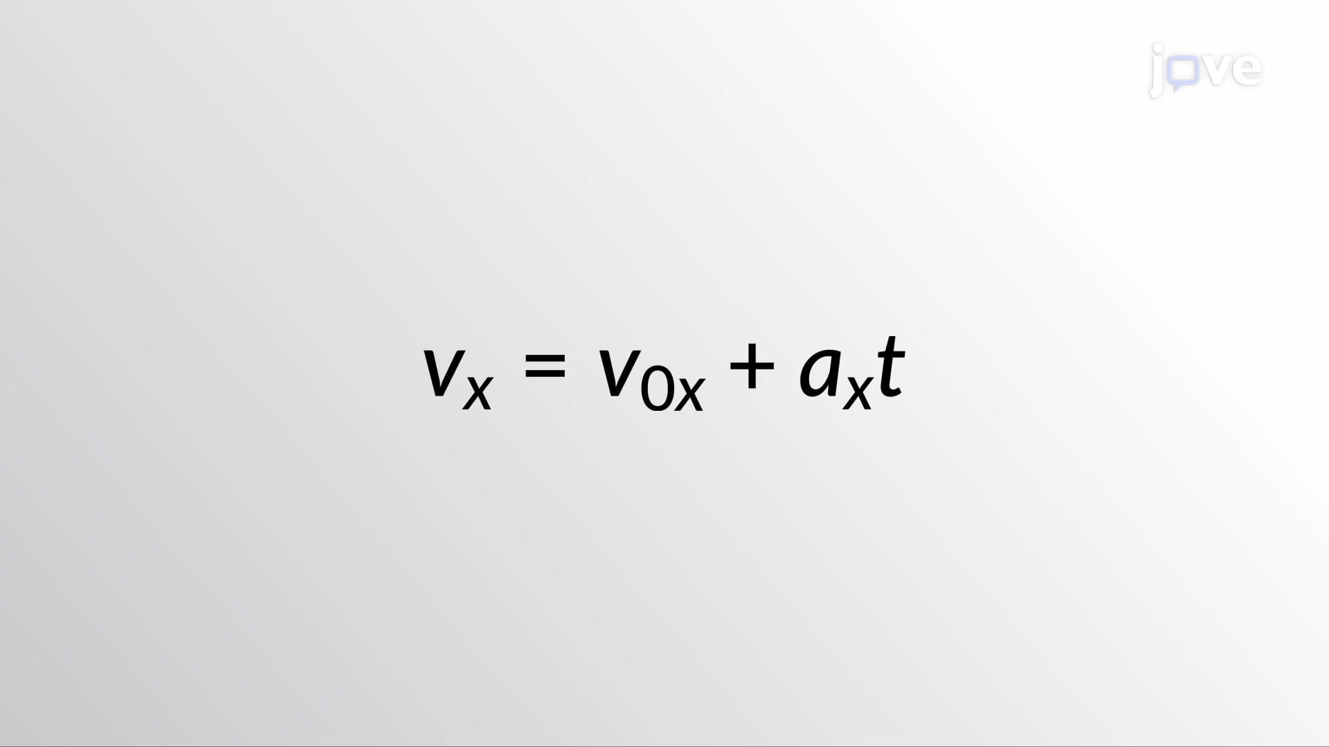
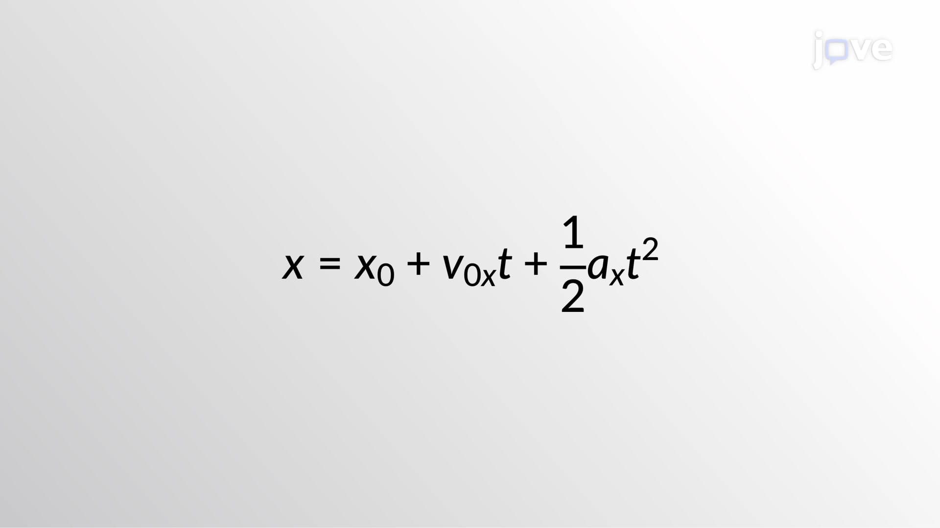
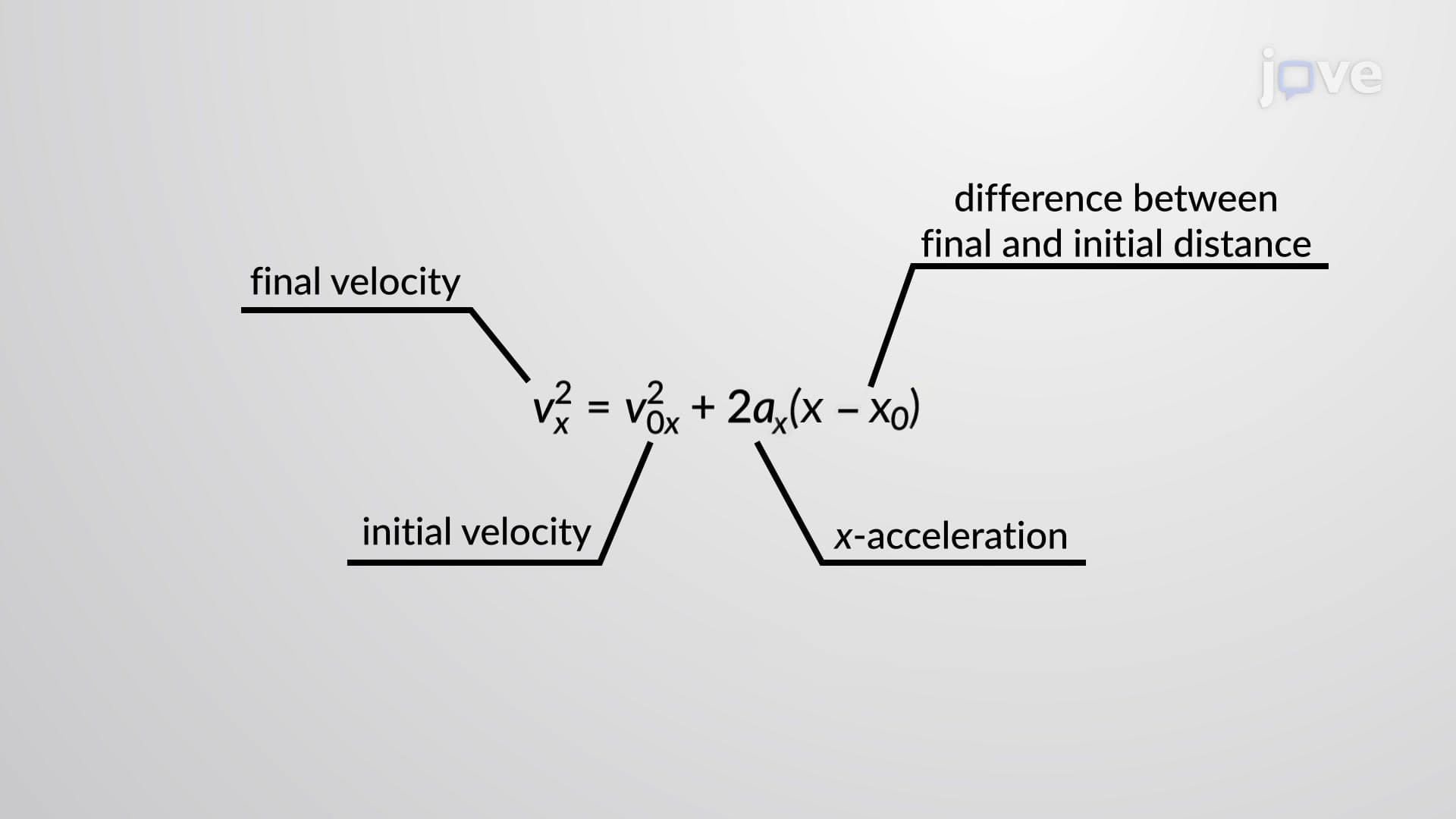
Loading video…


 14 Concepts
 224.2K views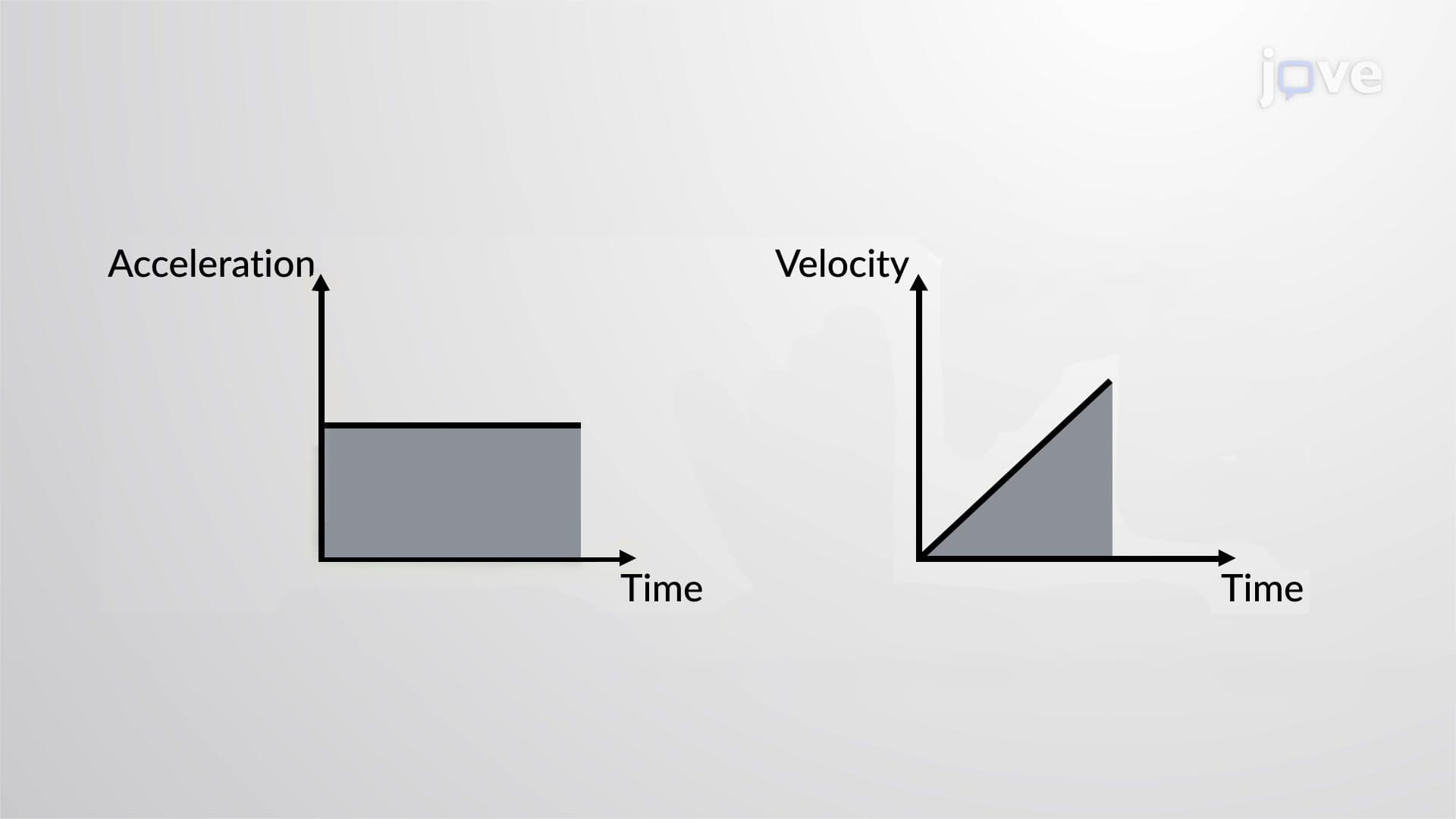

Video Summary: Velocity and Position by Graphical Method Guide
Ever wonder how NASA calculates a rocket's position during launch when acceleration constantly changes? The velocity and position by graphical method transforms complex motion into visual problem-solving by analyzing areas under curves. When studying acceleration-time graphs, the area underneath reveals velocity changes, while velocity-time graph areas show displacement-just like how engineers at SpaceX track their Falcon 9 rockets through atmospheric flight phases. Watch the full video on JoVE Coach to master this concept with expert-led visuals and step-by-step explanations.
The velocity and position by graphical method represents one of physics' most elegant problem-solving approaches, transforming abstract mathematical relationships into concrete visual analysis. This method becomes particularly powerful when dealing with non-uniform motion-situations where traditional kinematic equations fall short. Unlike constant acceleration scenarios taught in introductory physics, real-world motion often involves changing acceleration patterns that require sophisticated analytical tools.
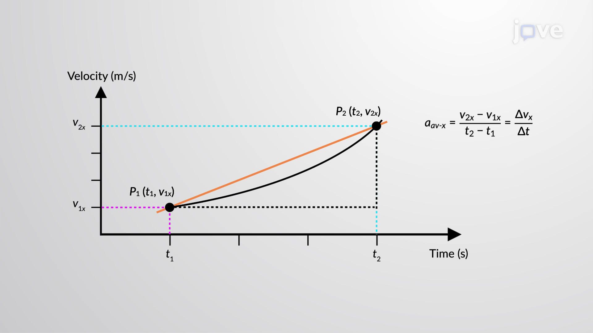
When acceleration varies with time, calculating velocity changes requires examining the area beneath acceleration-time graphs. Each rectangular strip represents a small time interval multiplied by average acceleration, yielding incremental velocity changes. For example, analyzing a car's acceleration during city driving involves multiple phases: initial acceleration from rest, coasting at constant speed, then deceleration for traffic lights. The cumulative area under this complex acceleration curve reveals total velocity change throughout the journey.
This rectangular approximation method mirrors techniques used in AP Physics courses and college-level mechanics. Students preparing for the MCAT encounter similar graphical analysis when studying physiological processes like cardiac output variations. The key insight involves recognizing that smaller time intervals (narrower rectangles) provide more accurate results, naturally leading toward integral calculus concepts.
Similarly, areas under velocity-time curves represent displacement or position changes. Consider analyzing a baseball's trajectory: the velocity-time graph shows initial upward velocity decreasing due to gravity, reaching zero at peak height, then becoming increasingly negative during descent. The total area-accounting for positive and negative regions-reveals net displacement from launch point.
This graphical approach proves invaluable for SAT Subject Test preparation and AP Physics exams, where students must interpret complex motion scenarios. Engineering students at universities like MIT and Stanford regularly apply these methods when analyzing mechanical systems, from oscillating springs to rotating machinery.
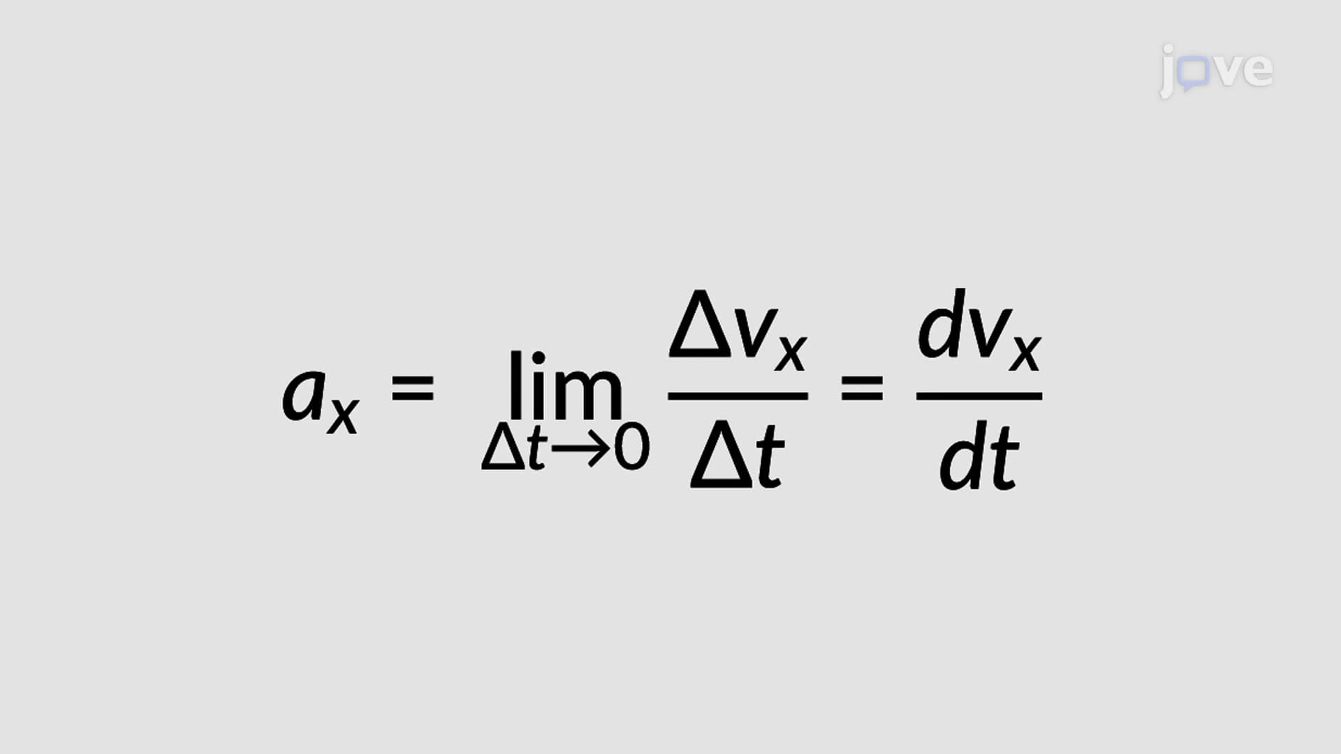
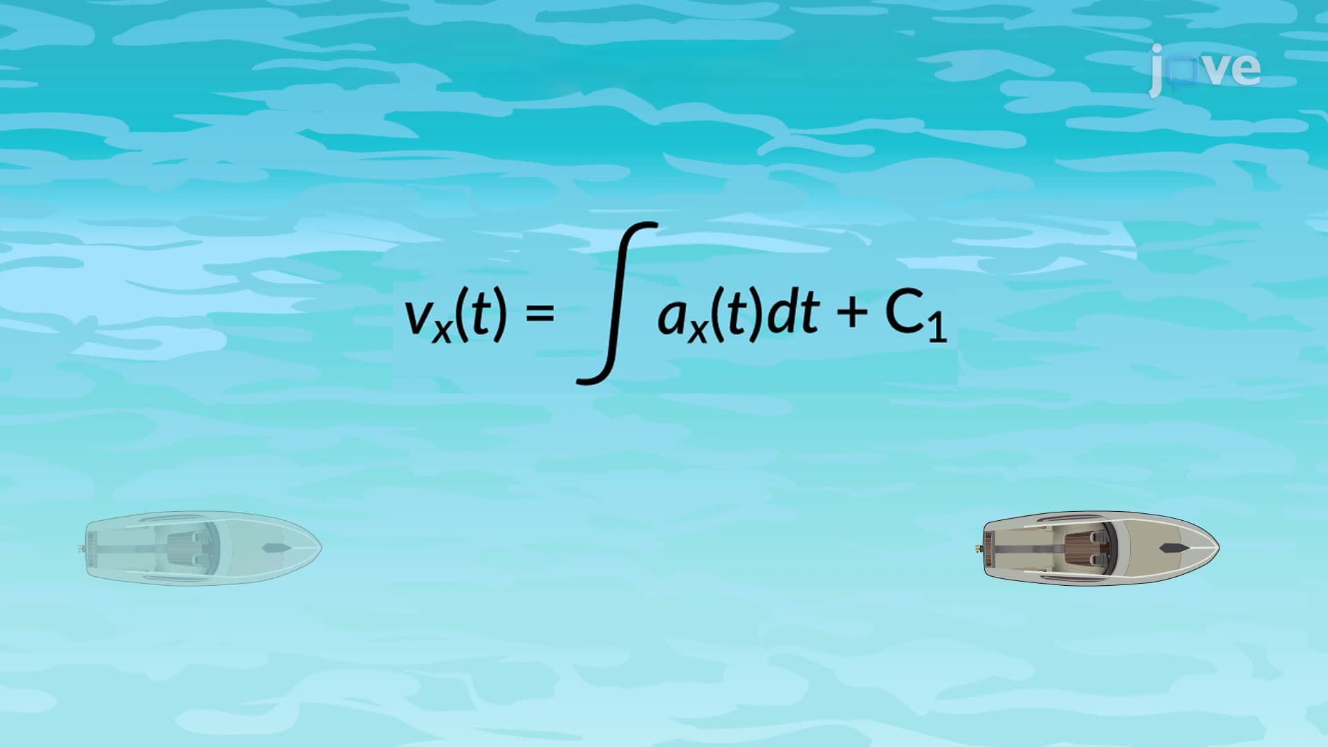
As time intervals approach zero, rectangular approximations transform into precise integral calculations. This transition illustrates calculus foundations emerging from geometric reasoning-a concept emphasized in advanced high school courses and college physics programs. The mathematical notation ∫a(t)dt for velocity change and ∫v(t)dt for displacement represents the logical endpoint of graphical methods, connecting visual problem-solving with analytical mathematics.
Related Micro-courses