Electrochemistry I: Electrolytic Conductance and Transference

Electrolytic conductance is central to understanding how ions carry electric current through solutions, a concept tested across AP Chemistry, MCAT, and college-level physical chemistry. This micro-course, supported by JoVE Coach, explores molar conductivity, transport numbers, Kohlrausch's law, Ostwald's dilution law, conductometric titrations, and the Debye-Hückel-Onsager equation, connecting fundamental electrochemical theory to real-world analytical and industrial applications.

• Understand the relationship between conductance, specific conductance, equivalent conductance, and molar conductivity, and how each quantity is measured and interpreted
• Learn how transport numbers and transference numbers quantify the contribution of individual ions to total current flow using Hittorf's and moving boundary methods
• Apply Kohlrausch's law to calculate molar conductivity at infinite dilution for weak electrolytes and sparingly soluble salts, including acetic acid and AgCl
• Analyze how concentration affects molar conductivity in both strong and weak electrolytes, and explain why these two classes behave differently upon dilution
• Identify the shapes and key intersection points in conductometric titration curves for strong acid-strong base, weak acid-strong base, and mixed acid systems
• Explore Ostwald's dilution law to determine the degree of dissociation of weak electrolytes, and understand why it fails for strong electrolytes like HCl and NaF
• Understand the ionic atmosphere model, including the asymmetry effect, electrophoretic effect, and viscous drag, and how they reduce molar conductivity at higher concentrations
• Apply the Debye-Hückel-Onsager equation to predict conductance behavior and interpret the Debye-Falkenhagen effect and Wien effect in strong electrolyte solutions

1. Electrolytic Conductance: From Resistance to Molar Conductivity

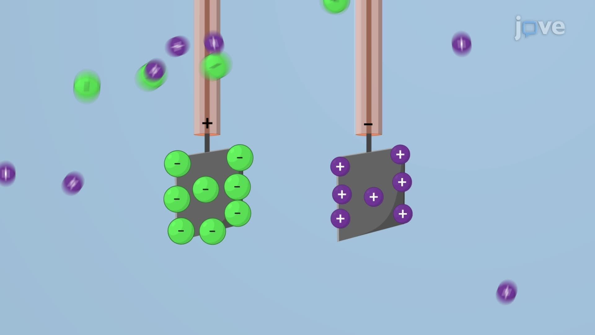
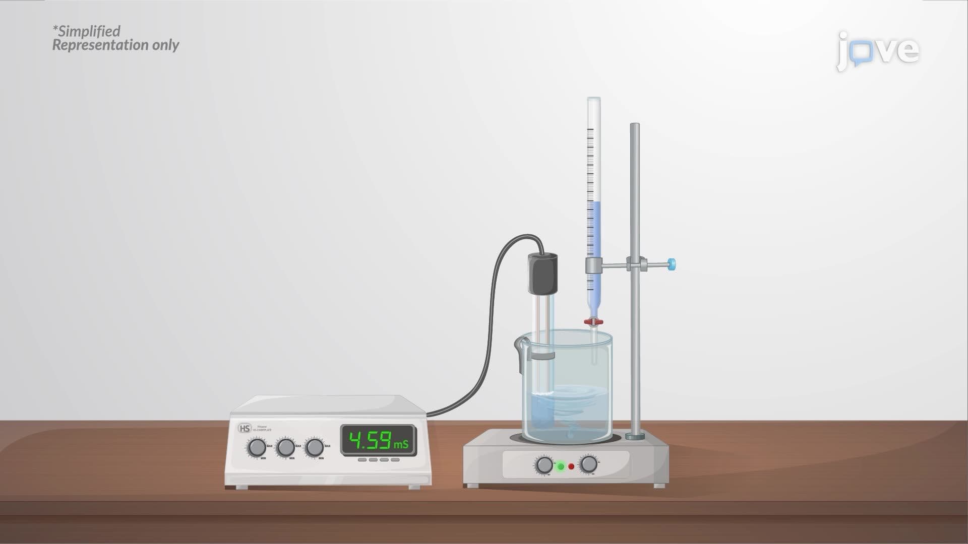
Conductance (G) is the inverse of resistance and measures how readily current flows through a solution. To make meaningful comparisons between solutions, the cell constant, the ratio of electrode separation to cross-sectional area, is used to calculate specific conductance (κ). Scaling further, equivalent conductance accounts for one gram equivalent of electrolyte, while molar conductivity (Λₘ) relates conductance to one mole of solute. A key trend: as dilution increases, Λₘ rises because electrolytes dissociate more completely, while κ falls because fewer ions per unit volume carry the current. Strong electrolytes approach a limiting value, molar conductivity at infinite dilution (Λₘ°), as concentration approaches zero.

2. Transport Number and Transference: Who Carries the Current?

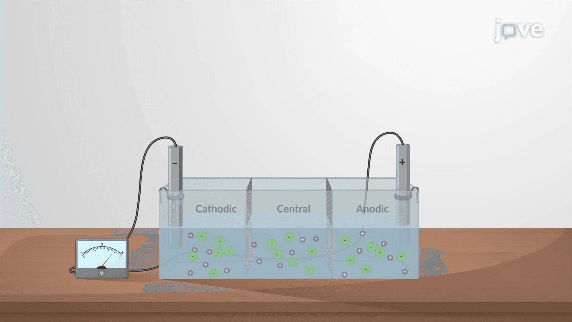
Not all ions contribute equally to current flow. The transference number (or transport number) quantifies the fraction of total current carried by each ion species. Hittorf's method tracks concentration changes in the anode, cathode, and central compartments of a divided cell to calculate this fraction. The ratio of cation mobility to anion mobility determines which ion dominates. The moving boundary method offers a more direct measurement: an applied potential shifts the visible boundary between two electrolytes (e.g., HCl and CdCl₂), and the displacement is used to calculate the transport number of H⁺ ions mathematically. Understanding transference numbers is essential in membrane science and electroplating.

3. Kohlrausch's Law and Its Applications

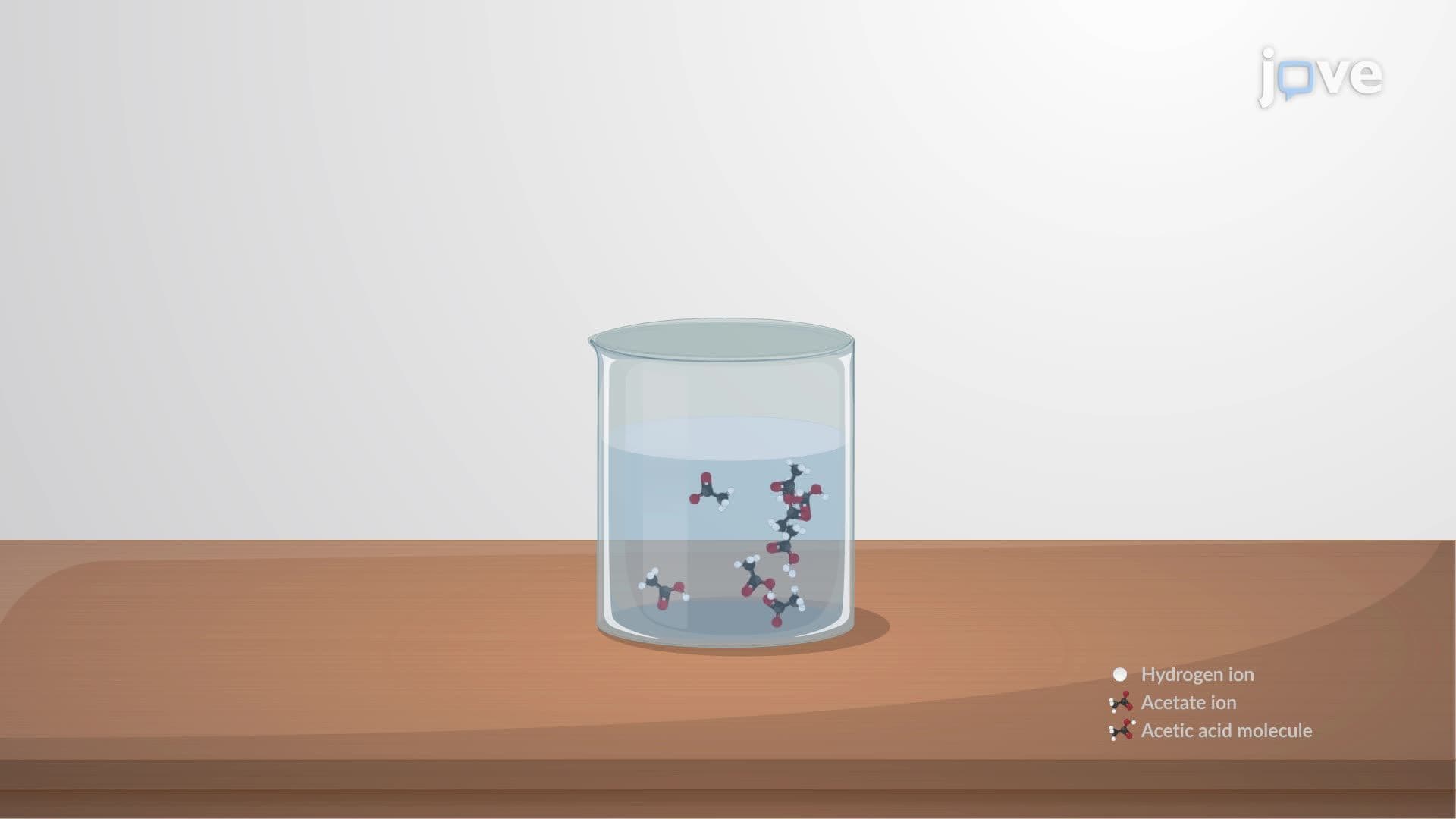
Kohlrausch's law states that, at infinite dilution, each ion contributes independently and additively to the total molar conductivity of an electrolyte, regardless of the identity of its counter-ion. Mathematically, Λₘ° = λ₊° + λ₋°, where λ° values are the molar ionic conductances at infinite dilution. This is particularly valuable for weak electrolytes like acetic acid, whose Λₘ° cannot be measured directly (since they never fully dissociate even at extreme dilution). By combining tabulated values, for example, adding Λₘ°(HCl) and Λₘ°(sodium acetate) then subtracting Λₘ°(NaCl), chemists can indirectly determine Λₘ° for acetic acid. The same strategy applies to sparingly soluble salts like AgCl. Kohlrausch's law also enables calculation of the degree of dissociation (α = Λₘ / Λₘ°).

4. Conductometric Titrations

Conductometric titrations exploit the fact that different ions have different mobilities, so replacing one ion with another changes solution conductance in predictable ways. In a strong acid-strong base titration (e.g., HCl with NaOH), fast H₃O⁺ ions are progressively replaced by slower Na⁺ ions, causing conductance to fall until neutralization; excess OH⁻ then raises conductance sharply. The endpoint appears as a V-shaped minimum. For a weak acid (e.g., acetic acid) titrated against NaOH, initial conductance is low due to incomplete dissociation; as highly ionized sodium acetate forms, conductance rises, then rises sharply again after the endpoint. Mixtures of strong and weak acids show three distinct linear segments. For strong acid-weak base (e.g., HCl and NH₄OH) systems, conductance drops then plateaus, since the weak base barely dissociates after neutralization. The titration endpoint in each case is identified at the intersection of straight-line segments on the conductance-vs-volume plot.

5. Ostwald's Dilution Law

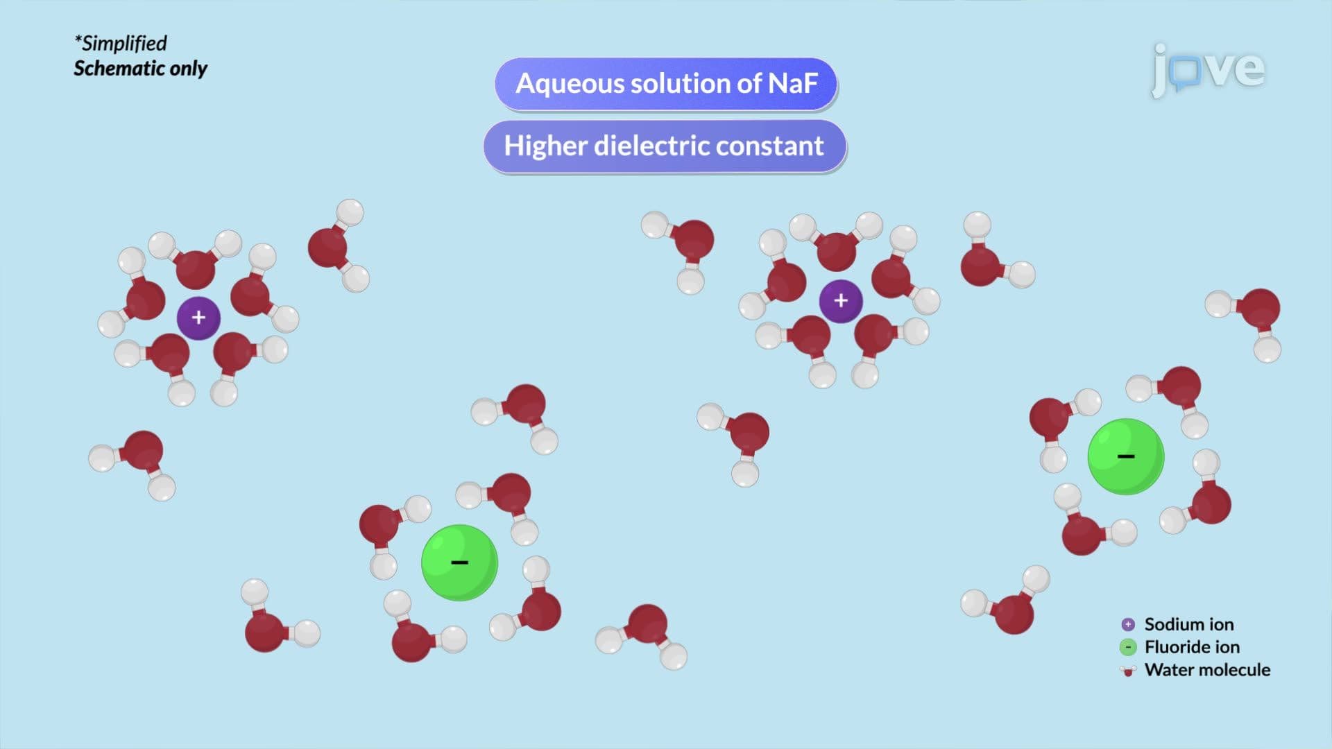
Derived from Arrhenius's theory of electrolytic dissociation, Ostwald's dilution law describes the equilibrium between undissociated molecules and ions in weak electrolyte solutions. For a weak electrolyte AB at concentration c with degree of dissociation α, the dissociation constant is expressed as K = cα² / (1 − α). This allows chemists to calculate α for weak electrolytes like acetic acid or NH₄OH at any concentration. Critically, this law does not apply to strong electrolytes like HCl or NaF. Water's high dielectric constant neutralizes interionic attractions, causing complete dissociation, meaning no undissociated molecules exist in equilibrium, and the mathematical expression becomes invalid. Recognizing this boundary is a common exam focus.

6. Theory of Strong Electrolytes and the Debye-Hückel-Onsager Equation

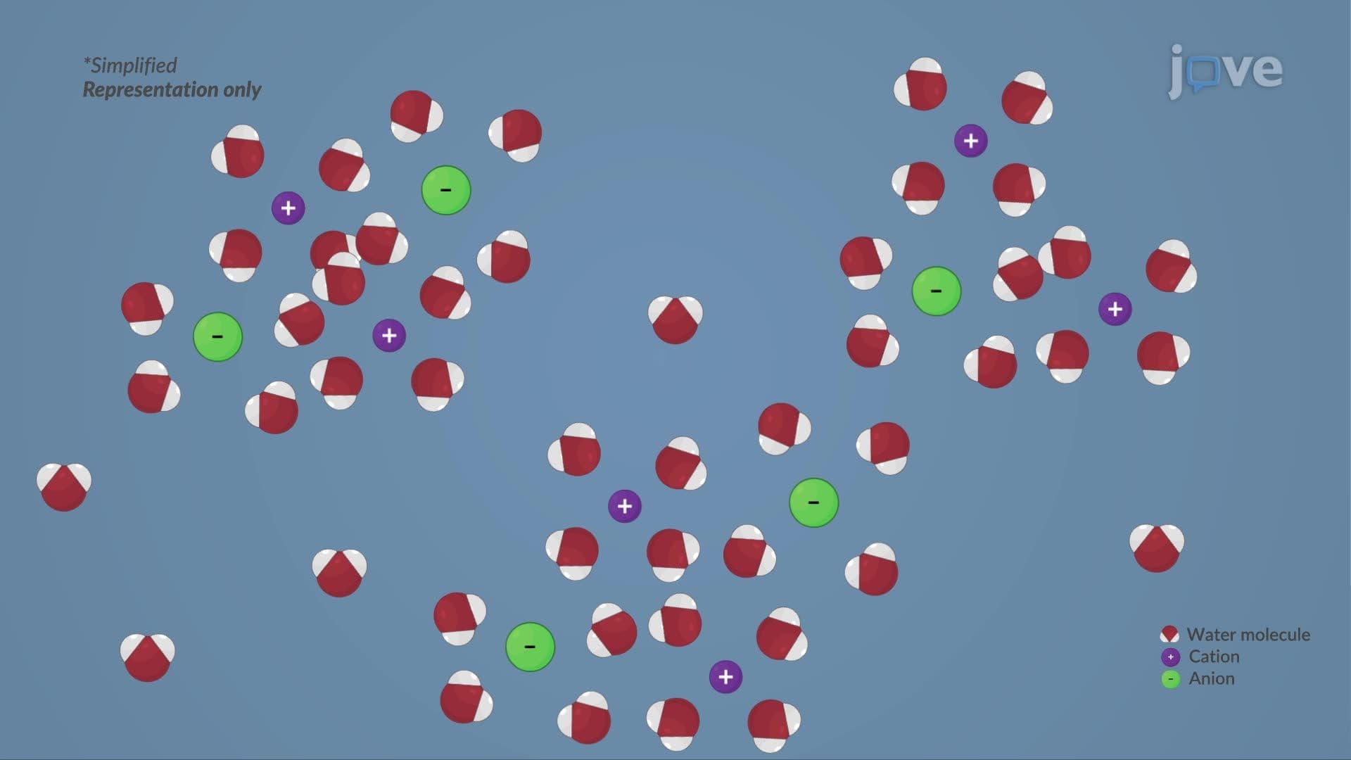
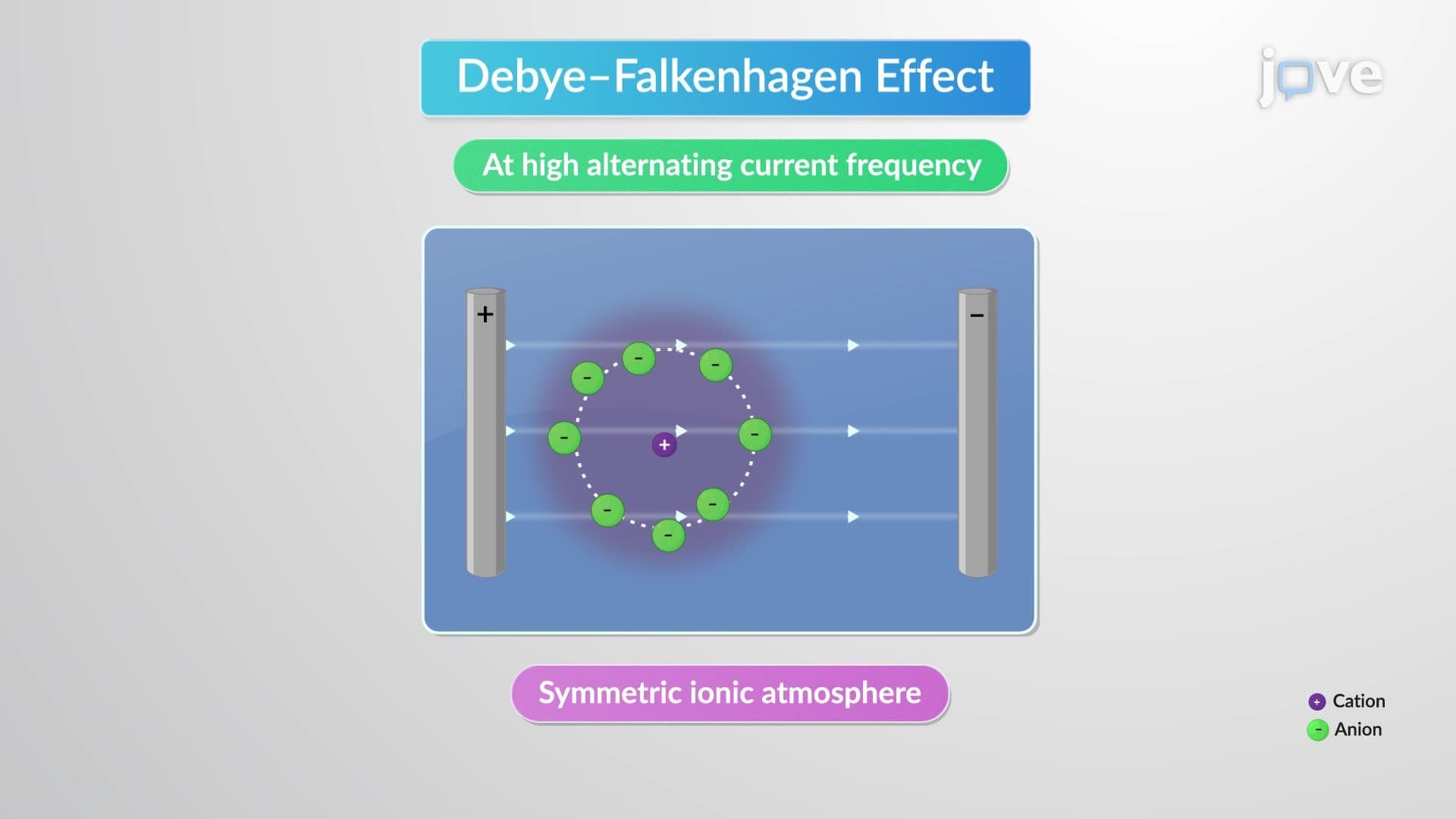
Strong electrolytes are fully ionized at all concentrations up to saturation. Yet Λₘ decreases with increasing concentration, a finding explained by interionic interactions. Each ion is surrounded by an "ionic atmosphere" of opposite charges. When an electric field is applied, two retarding effects emerge: the asymmetry (relaxation) effect, where the ionic atmosphere lags behind the moving central ion, and the electrophoretic effect, where the surrounding solvent and ionic cloud move counter to the ion. Together with viscous drag, these effects reduce ionic mobility. The Debye-Hückel-Onsager equation formalizes this: Λₘ = Λₘ° − (A + BΛₘ°)√c, predicting a linear plot of Λₘ vs. √c, experimentally confirmed for uni-univalent electrolytes. The Debye-Falkenhagen effect (conductance increases with AC frequency) and the Wien effect (conductance increases at high field strength) further validate this model.