Loading video…

 16 Concepts
 51 views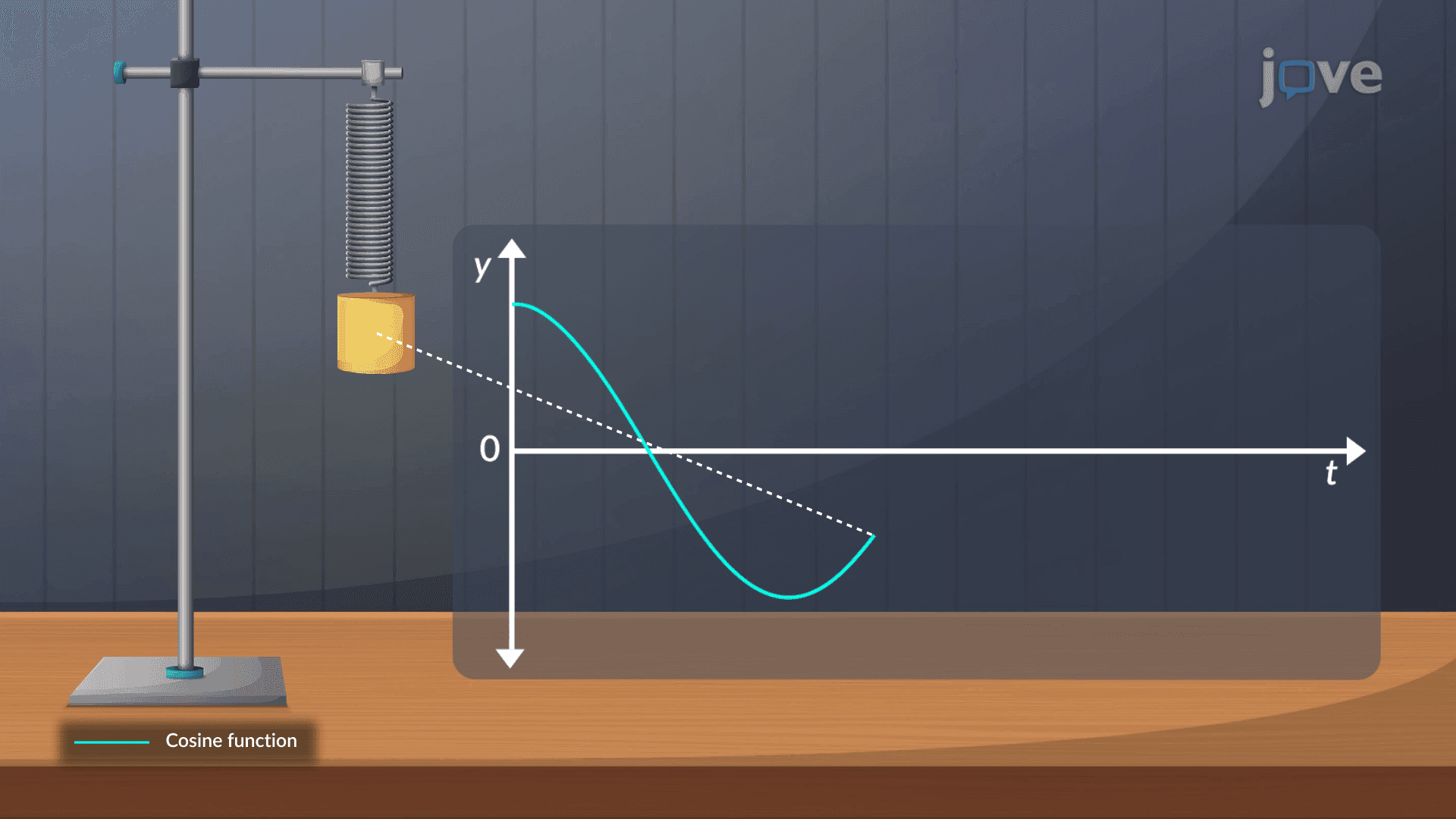

Video Summary: What are Applications of Taylor Series
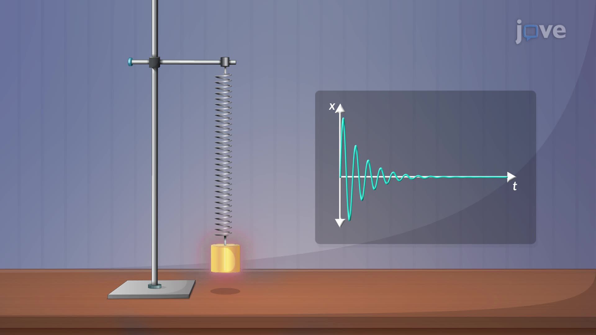
Ever wonder how a video game engine calculates smooth physics in real time without crashing your CPU? The applications of Taylor series make that possible. What are Applications of Taylor Series? They allow engineers and scientists to replace complex functions with simpler polynomial approximations, like modeling a mass-spring system in introductory physics at MIT or Caltech. Watch the full video on JoVE Coach to master this concept with expert-led visuals and step-by-step explanations.
The applications of Taylor series reach far beyond the walls of a calculus classroom. At their core, Taylor series allow mathematicians, physicists, and engineers to rewrite complicated functions, trigonometric, exponential, logarithmic, as infinite sums of polynomial terms. Polynomials are easy to compute, differentiate, and integrate, making this substitution incredibly powerful. Whether you are studying AP Calculus BC, taking Calculus II at a state university, or preparing for a physics or engineering program, Taylor series will appear repeatedly throughout your academic career.
When a Taylor series is built around the center point x = 0, it is called a Maclaurin series. This special case produces a cleaner form because every term is a power of x evaluated using derivatives at zero. Common Maclaurin series, for functions like sin(x), cos(x), and e^x, are so frequently used in physics and engineering that students are expected to memorize them for exams like AP Calculus BC and college midterms. For example, the cosine Maclaurin series begins: cos(x) ≈ 1 − x²/2! + x⁴/4! − x⁶/6! + … Each additional term captures more of the function's oscillatory shape.
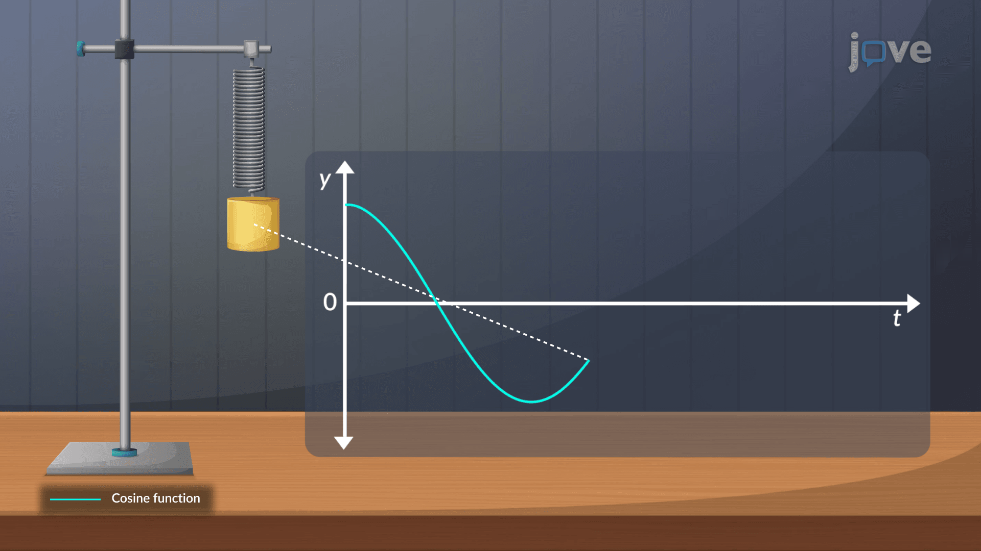
One of the most concrete applications of Taylor series appears in modeling simple harmonic motion, the back-and-forth movement of a mass attached to a spring. Describing this motion requires a cosine function, which is computationally expensive for processors to evaluate repeatedly at high speeds. In aerospace simulations run by organizations like NASA's Jet Propulsion Laboratory (JPL), or in real-time physics engines used by US video game developers, programmers substitute the full cosine function with its Maclaurin approximation. For small time values close to the starting point, just two or three terms deliver excellent accuracy while dramatically reducing processing load. This is a direct, practical payoff of understanding power series in an applied context.
A Taylor series is only useful within its interval of convergence, the range of input values where the series actually approaches the correct function value. Outside this range, the series may diverge and give wildly incorrect results. To find the interval of convergence of a power series, students apply convergence tests such as the ratio test, the root test, or the alternating series test. On AP Calculus BC exams and college Calculus II midterms, these tests appear frequently, so mastering them is essential. It is also worth understanding how Taylor series relates to geometric series, in fact, the geometric series 1/(1−x) is itself a simple power series, and recognizing that connection builds intuition for convergence behavior.
Students sometimes ask: what is the difference between a sequence and a series? A sequence is an ordered list of numbers (like 1, 1/2, 1/4, 1/8, …), while a series is the sum of a sequence's terms (1 + 1/2 + 1/4 + 1/8 + …). Taylor series are infinite series built from a specific rule tied to a function's derivatives. Understanding this distinction helps students correctly set up convergence tests and interpret what a Taylor approximation is actually computing. In US college courses like Calculus II or Mathematical Methods for Engineers, this conceptual clarity is often tested directly on quizzes and exams.
Related Micro-courses