Loading video…

 19 Concepts
 5.7K views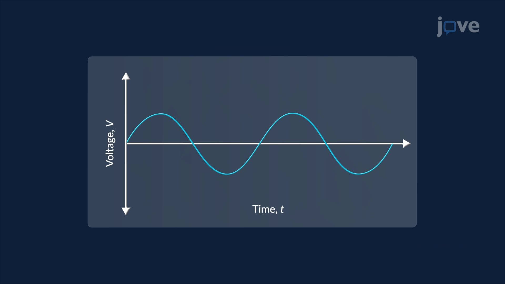

Video Summary: Absolute and Local Extreme Values Explained
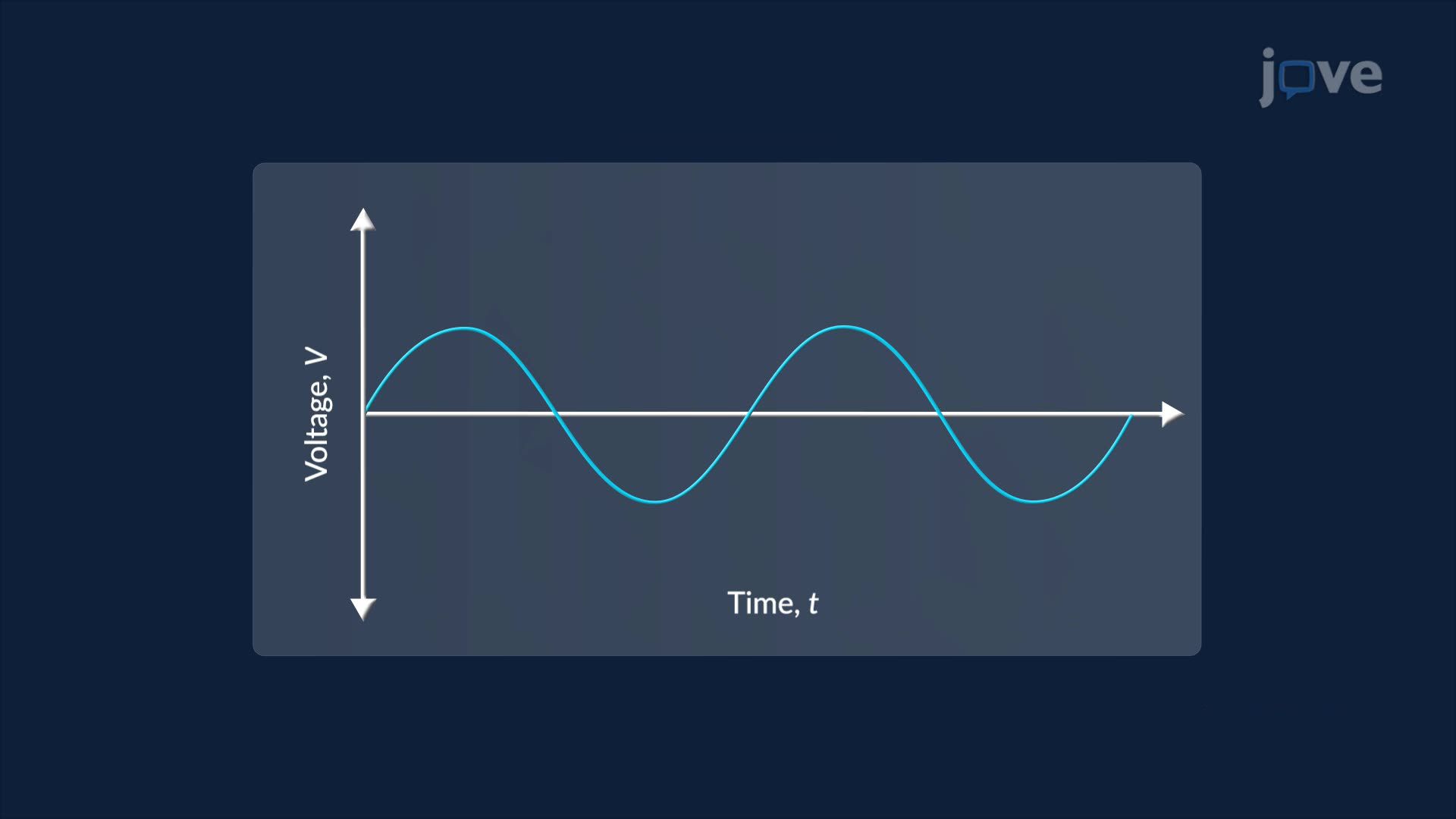
Did you know that electrical engineers use calculus to keep your phone charger from overheating? Understanding absolute and local extreme values, the core idea behind Absolute and Local Extreme Values Explained, is exactly how they do it. The Extreme Value Theorem guarantees that any continuous function on a closed interval has both a highest and lowest point, whether you're tracking daily temperatures in Chicago or voltage cycles in a circuit. Watch the full video on JoVE Coach to master this concept with expert-led visuals and step-by-step explanations.
When you study calculus, few ideas are as practically powerful as Absolute and Local Extreme Values Explained. These concepts allow mathematicians, engineers, economists, and scientists to pinpoint exactly where a function reaches its highest or lowest output, and that information drives everything from drug dosage optimization in US hospitals to maximizing profit margins in business models.
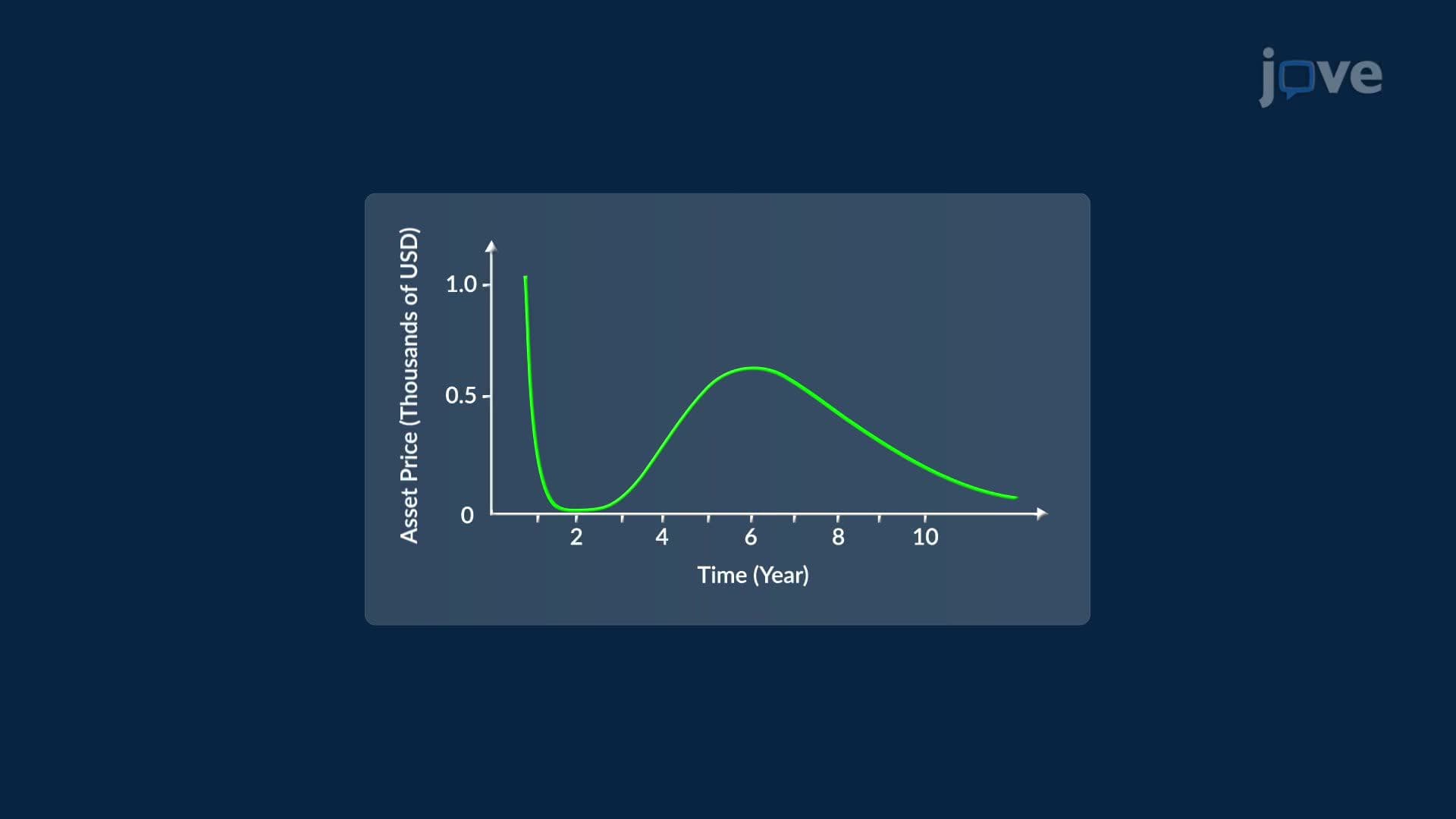
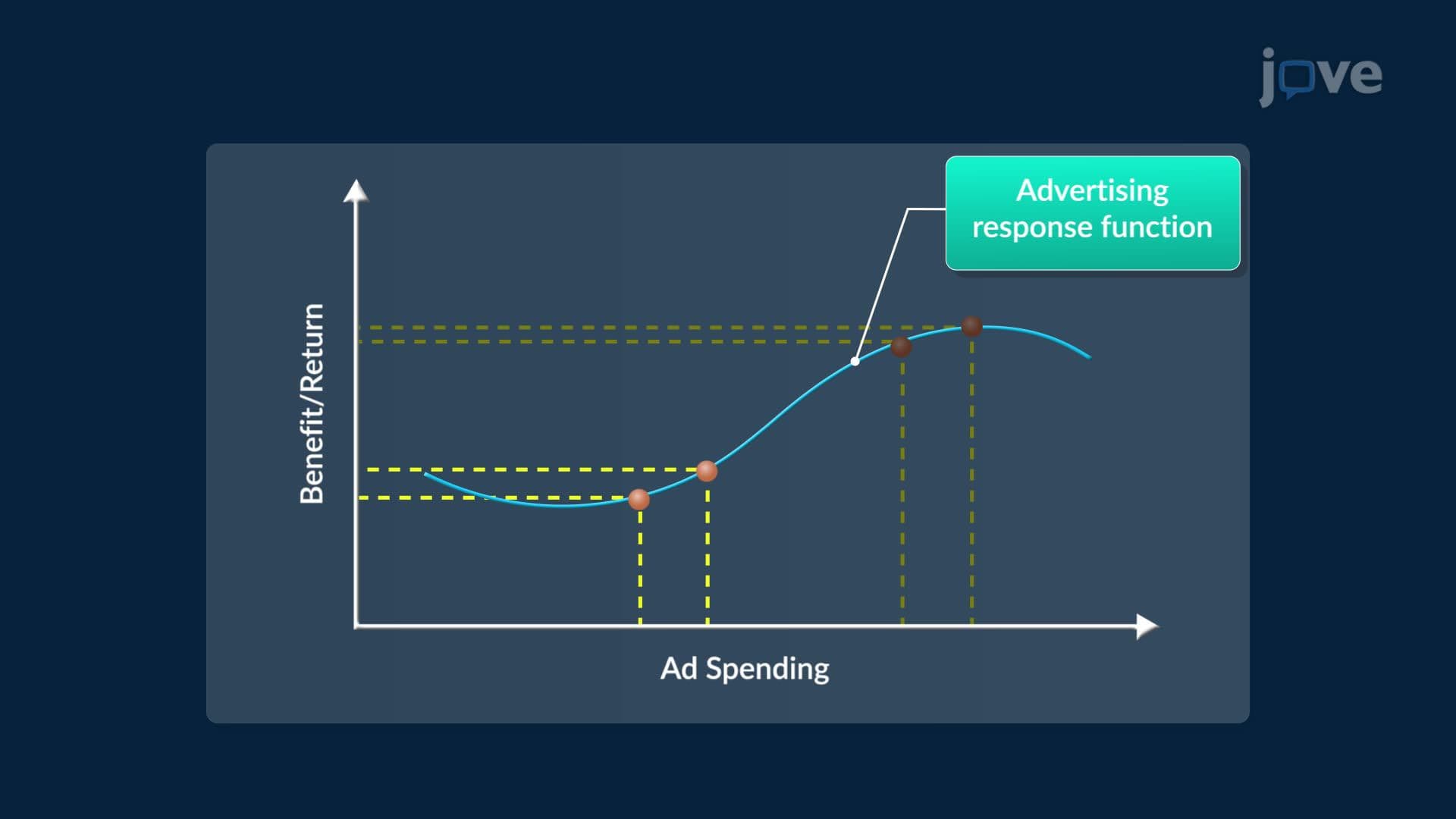
An absolute maximum (also called a global maximum) is the single largest value a function achieves over its entire domain or a specified interval. An absolute minimum is the smallest. In contrast, a local maximum (or relative maximum) is a point where the function value is higher than all nearby points, but not necessarily the highest overall. The same logic applies to a local minimum.
The Extreme Value Theorem is the foundation here. It states: if a function is continuous on a closed interval [a, b], then it must attain both an absolute maximum and an absolute minimum somewhere on that interval. This is not just a suggestion, it is a mathematical guarantee.
The word *closed* is critical. Open intervals or discontinuous functions do not carry this guarantee. For example, the function f(x) = 1/x on the open interval (0, 1) has no absolute maximum because the function grows without bound near x = 0.
To find absolute extreme values on a closed interval [a, b], follow these three steps:
1. Find the derivative of the function, f'(x). 2. Locate critical points, values of x where f'(x) = 0 or f'(x) is undefined, and which lie within the interval. 3. Evaluate the function at each critical point and at both endpoints (x = a and x = b).
The largest output is the absolute maximum; the smallest is the absolute minimum. This method is routinely tested on the AP Calculus AB and BC exams, and mastering it is essential for college midterms in Calculus I and II.
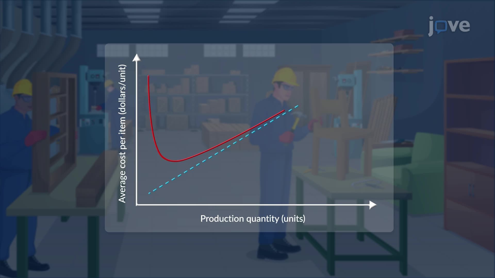
For example, a NASA mission planning team modeling fuel consumption over a fixed flight window uses exactly this method, they evaluate a continuous cost function at critical points and endpoints to find the most and least efficient burn rates.
Understanding local extrema also requires knowing the First and Second Derivative Tests. The First Derivative Test checks whether f'(x) changes sign around a critical point, if it goes from positive to negative, you have a local maximum; negative to positive indicates a local minimum.
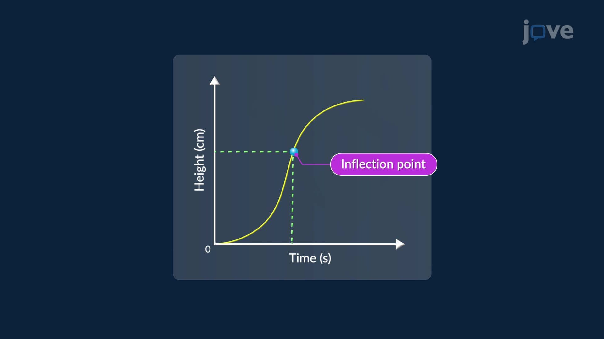
The Second Derivative Test uses concavity: if f''(x) < 0 at a critical point, the curve is concave down, a local maximum. If f''(x) > 0, the curve is concave up, a local minimum. Points where concavity changes are called inflection points, and they are closely related to optimization problems across physics, economics, and engineering.
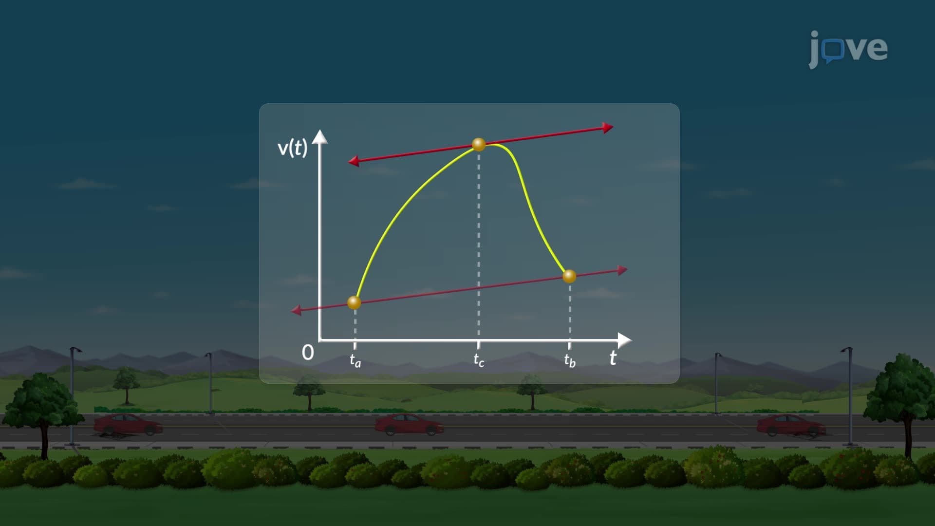
These tools also connect directly to the Mean Value Theorem, which guarantees at least one point where the instantaneous rate of change equals the average rate of change over an interval, a concept that appears in both AP Calculus FRQs and college-level proofs.
Related Micro-courses