Loading video…

 19 Concepts
 5.7K views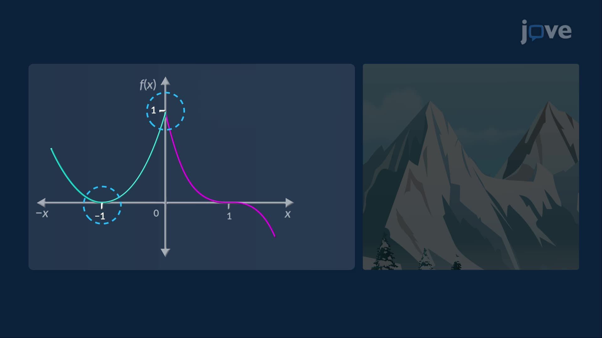

Video Summary: Critical Numbers and the Closed Interval Method Guide
Did you know that engineers designing roller coasters use the same calculus concept that helps students ace AP exams? Critical numbers and the closed interval method basics reveal exactly where functions hit their highest and lowest values, essential for solving optimization problems. NASA engineers, for instance, use this approach to minimize fuel consumption on flight paths. Watch the full video on JoVE Coach to master this concept with expert-led visuals and step-by-step explanations.
One of the most powerful tools in calculus is the ability to pinpoint exactly where a function reaches its peak or its lowest point. Whether you are a student working through AP Calculus AB or an engineering undergraduate solving real design problems, critical numbers and the closed interval method form the bedrock of this skill. Understanding these ideas deeply, not just mechanically, transforms how you approach entire categories of problems.
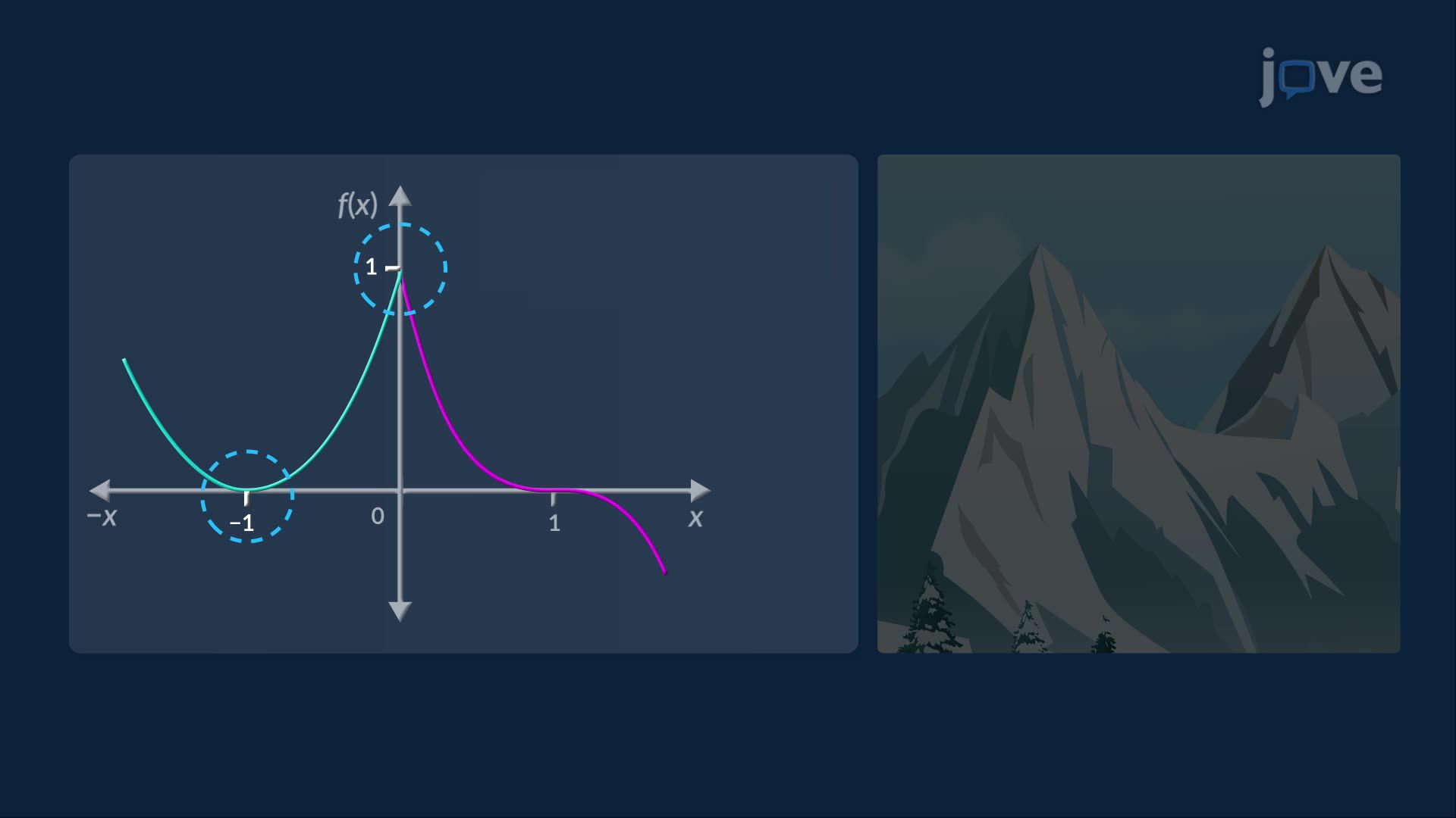
A critical number is any value in a function's domain where the derivative is either equal to zero or fails to exist. These two conditions capture every possible candidate for a local high or low point. Fermat's Theorem formalizes this: if a function has a local maximum or minimum at a point and the derivative exists there, then the derivative must equal zero at that point. Crucially, the converse is not automatically true, a derivative equal to zero does not guarantee an extremum. For example, f(x) = x³ has a derivative of zero at x = 0, yet that point is neither a local max nor a local min.
Sharp corners and cusps, common in absolute value functions like f(x) = |x|, represent points where the derivative is undefined. Even so, a local minimum clearly exists at x = 0 for that function. This nuance often trips up students on AP Calculus exams, making it essential to check both conditions every time.
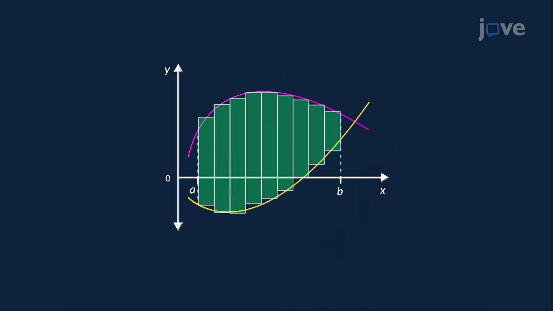
When a continuous function is defined on a closed interval [a, b], the Extreme Value Theorem guarantees that absolute maximum and minimum values exist. The Closed Interval Method provides a reliable, step-by-step way to find them:
1. Find all critical numbers that lie strictly inside the open interval (a, b), that is, where the derivative is zero or undefined. 2. Evaluate the function at each of those critical numbers. 3. Evaluate the function at both endpoints, f(a) and f(b).
The largest value from all these evaluations is the absolute maximum; the smallest is the absolute minimum. This method works because, on a closed interval, extreme values can only occur at critical numbers or at the boundary endpoints, nowhere else.
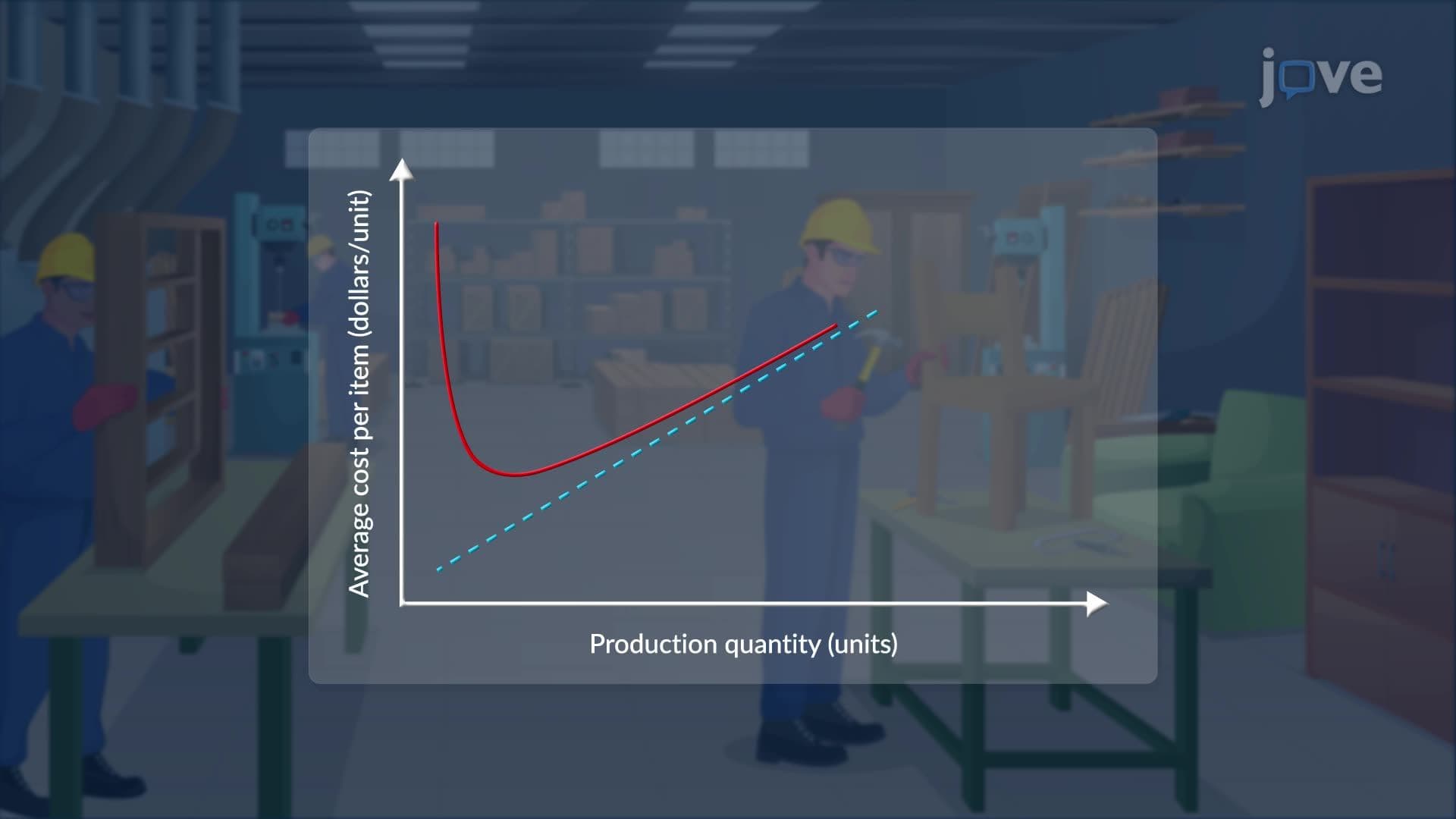
This method appears constantly in applied settings across the United States. A civil engineering team designing a highway overpass might model the load on a beam as a function and use the Closed Interval Method to find the point of maximum stress within a fixed span length. In business calculus courses at universities like UCLA or the University of Michigan, students use the same approach to minimize production costs or maximize revenue over a defined output range. Even in AP Calculus, free-response questions frequently ask students to justify absolute extrema on a closed interval, and the College Board specifically rewards work that checks both critical numbers and endpoints.
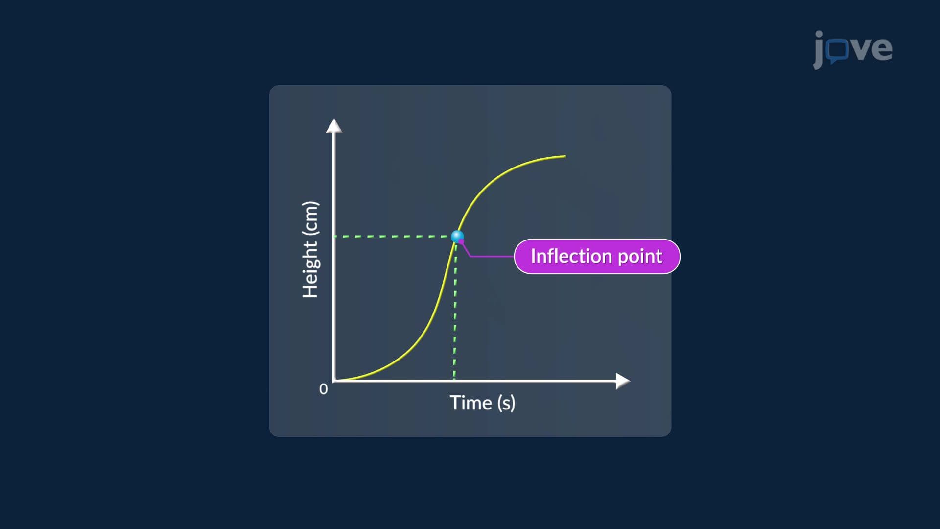
Critical numbers do not exist in isolation. They serve as the entry point into curve sketching, where the first derivative test reveals whether a critical number produces a local max, local min, or neither. They connect directly to concavity and inflection points through the second derivative, and they appear in Mean Value Theorem discussions about where a derivative takes a specific value. For students heading into multivariable calculus or differential equations, the logic of identifying and testing critical points scales naturally into higher dimensions. Mastering this concept now creates a durable framework that pays dividends throughout an entire STEM education.
Related Micro-courses