Loading video…

 19 Concepts
 5.7K views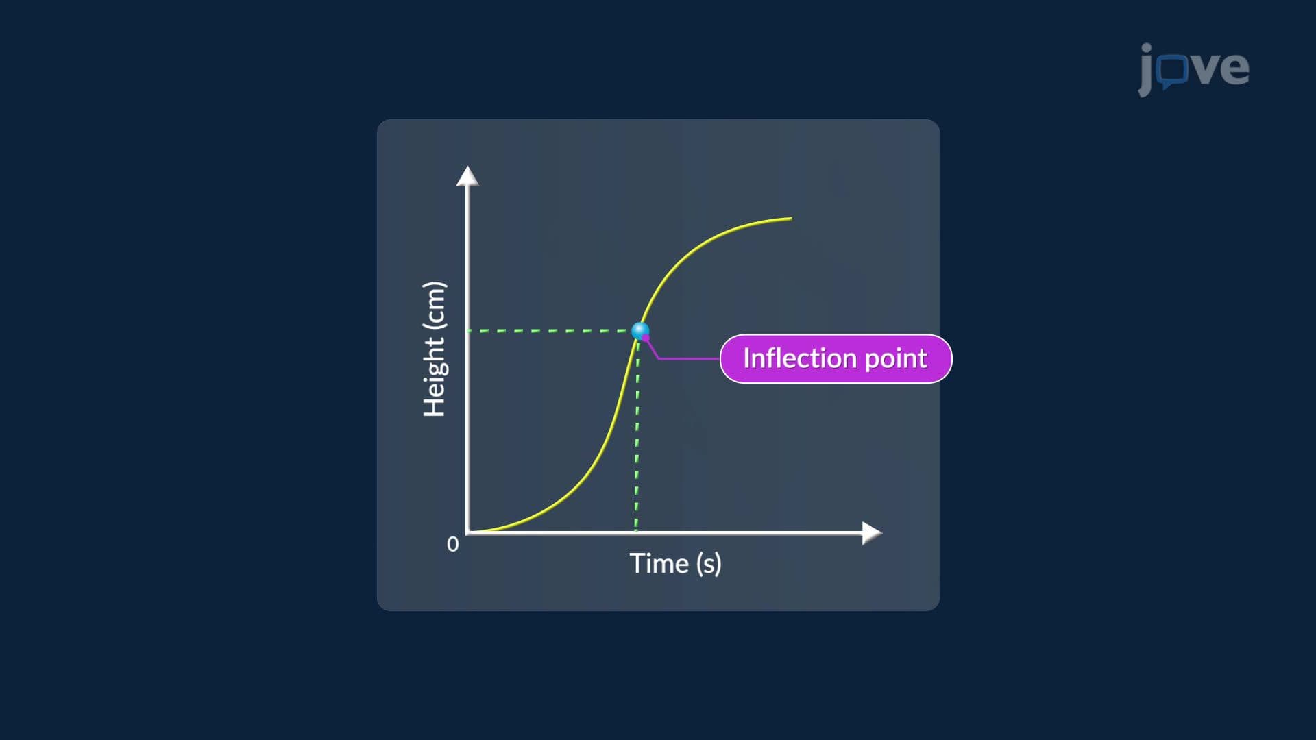

Video Summary: Problem Solving in Second Derivative Test
Did you know a coffee mug can teach you calculus? Problem Solving in Second Derivative Test becomes intuitive when you analyze how liquid rises in a mug with a curved shape, wider at top and bottom, narrow in the middle. The second derivative reveals whether the rise accelerates or decelerates, pinpointing inflection points where concavity shifts. Watch the full video on JoVE Coach to master this concept with expert-led visuals and step-by-step explanations.
The second derivative test is one of the most powerful tools in calculus, not just for passing exams, but for understanding how real systems behave. Whether you are analyzing the path of a roller coaster at Six Flags, modeling population growth for a biology course, or solving optimization problems on the AP Calculus AB exam, the second derivative gives you critical information about how a function is changing. Mastering problem solving in second derivative test basics means learning to read that information fluently.
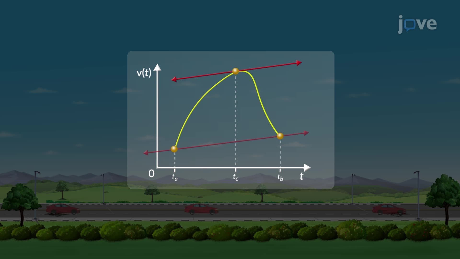
Most students know the first derivative tells you slope, whether a function is increasing or decreasing. The second derivative goes one level deeper: it measures how the slope itself is changing. In mathematical terms, if f''(x) > 0, the slope is increasing, which means the curve bends upward (concave up). If f''(x) < 0, the slope is decreasing, and the curve bends downward (concave down). Think of it like driving: the first derivative is your speed, and the second derivative is your acceleration. A positive second derivative means you are speeding up; a negative one means you are slowing down.
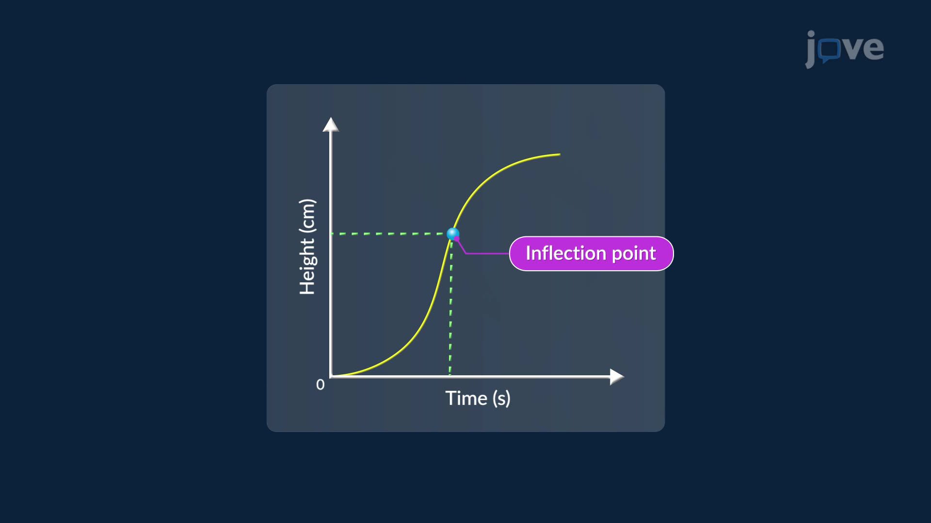
An inflection point occurs where the second derivative equals zero AND changes sign. This is not just a mathematical technicality, it marks a meaningful transition in the real world. In the classic mug example, the inflection point sits at the narrowest part of the mug, where the cross-sectional area is smallest. Below that point, the liquid level rises with increasing speed (concave up). Above it, the liquid level continues to rise but with decreasing speed (concave down). The second derivative transitions from positive to negative, passing through zero exactly at the inflection point. Students frequently confuse f''(x) = 0 with an automatic inflection point, always verify the sign change.
The second derivative test shines brightest when combined with optimization problems. Once you locate a critical point where f'(x) = 0, the second derivative tells you what type of critical point it is. If f''(x) > 0 at that point, it is a local minimum. If f''(x) < 0, it is a local maximum. If f''(x) = 0, the test is inconclusive and you must use other methods, such as the first derivative test. This application appears frequently on the AP Calculus BC free-response section, college midterms, and in engineering coursework where maximizing efficiency or minimizing cost is essential, for example, designing a fuel-efficient aircraft wing profile.
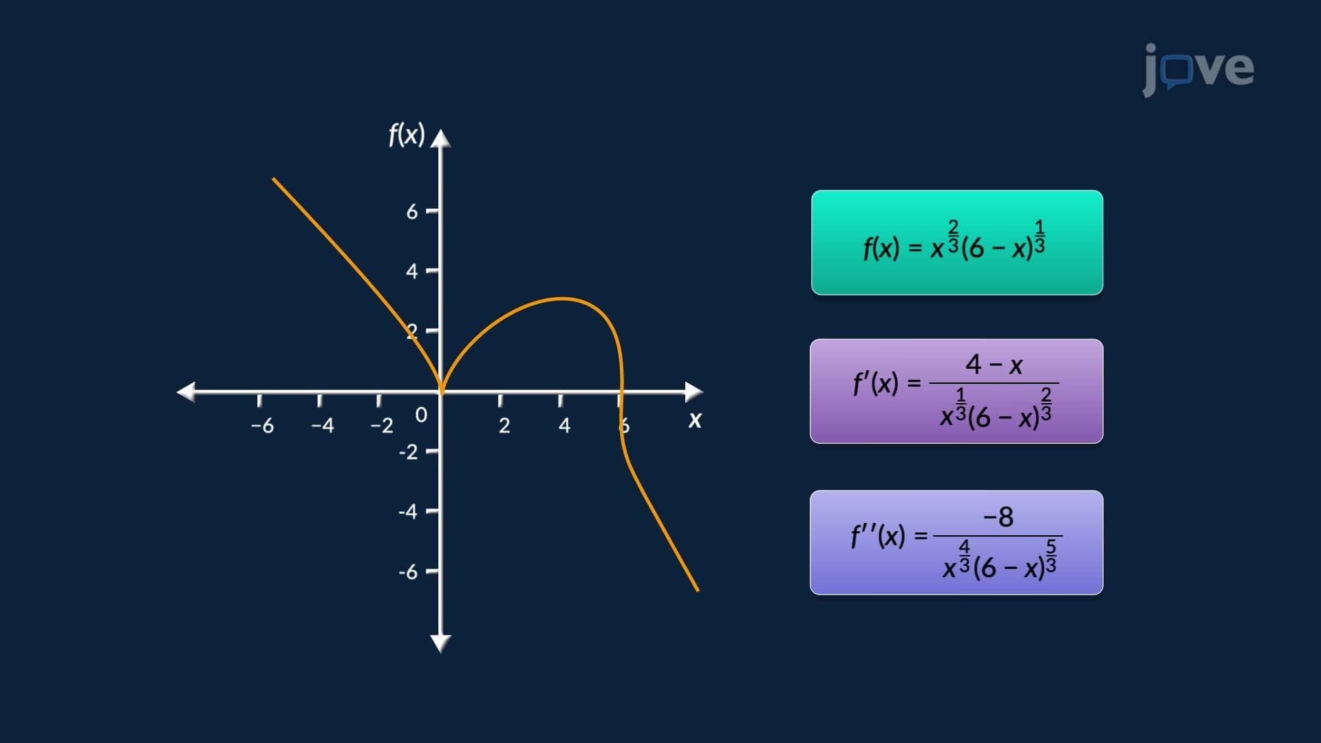
In AP Calculus and college courses across the United States, curve sketching tasks require students to synthesize information from both the first and second derivatives. You must identify intervals of increase or decrease, locate maximum and minimum values, determine concavity, and mark inflection points, all in one coherent analysis. Related rates problems, another core topic, sometimes involve the second derivative when the question asks not just how fast something changes, but whether that change is accelerating or slowing. The Mean Value Theorem also provides foundational logic here: it guarantees that the instantaneous rate of change matches the average rate somewhere on an interval, connecting smoothly to how the second derivative behaves across that same region. Practicing structured problem solving in second derivative test scenarios, especially with physical, visual models, dramatically improves both conceptual understanding and exam performance.
Related Micro-courses