Loading video…


 19 Concepts
 5.7K views

Video Summary: The Antiderivative of a Function Explained
Ever wonder how engineers at NASA calculate a rocket's position when they only know its velocity? The antiderivative of a function is the key mathematical tool that makes this possible. Understanding the antiderivative of a function basics lets you reverse the differentiation process to recover original functions from their rates of change. Watch the full video on JoVE Coach to master this concept with expert-led visuals and step-by-step explanations.
The antiderivative of a function is a foundational concept in calculus that answers a deceptively simple question: if you know how something is changing, can you figure out what it was? In formal terms, a function F(x) is called an antiderivative of f(x) if the derivative of F(x) equals f(x). This operation, working backward from a derivative to its original function, is the starting point for integral calculus and appears across AP Calculus AB, AP Calculus BC, and college-level Calculus I courses nationwide.
One of the most important, and most frequently misunderstood, aspects of antiderivatives is that they are not unique. Consider the functions x², x² + 7, and x² − 12. All three have the same derivative: 2x. This happens because the derivative of any constant is zero, meaning constant information is permanently erased during differentiation. To account for every possible function that could have produced a given derivative, mathematicians write the general antiderivative as F(x) + C, where C represents the arbitrary constant of integration. Omitting C on an AP Calculus free-response question is a common error that costs students points, even when the rest of the work is correct.
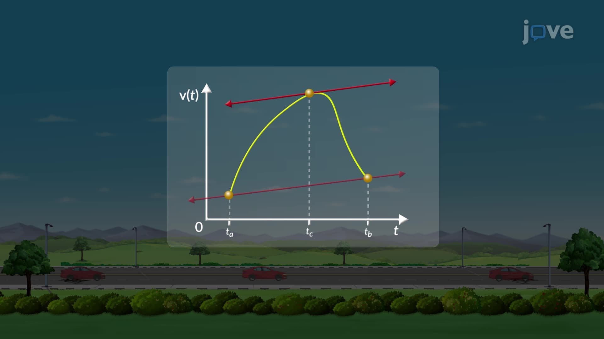
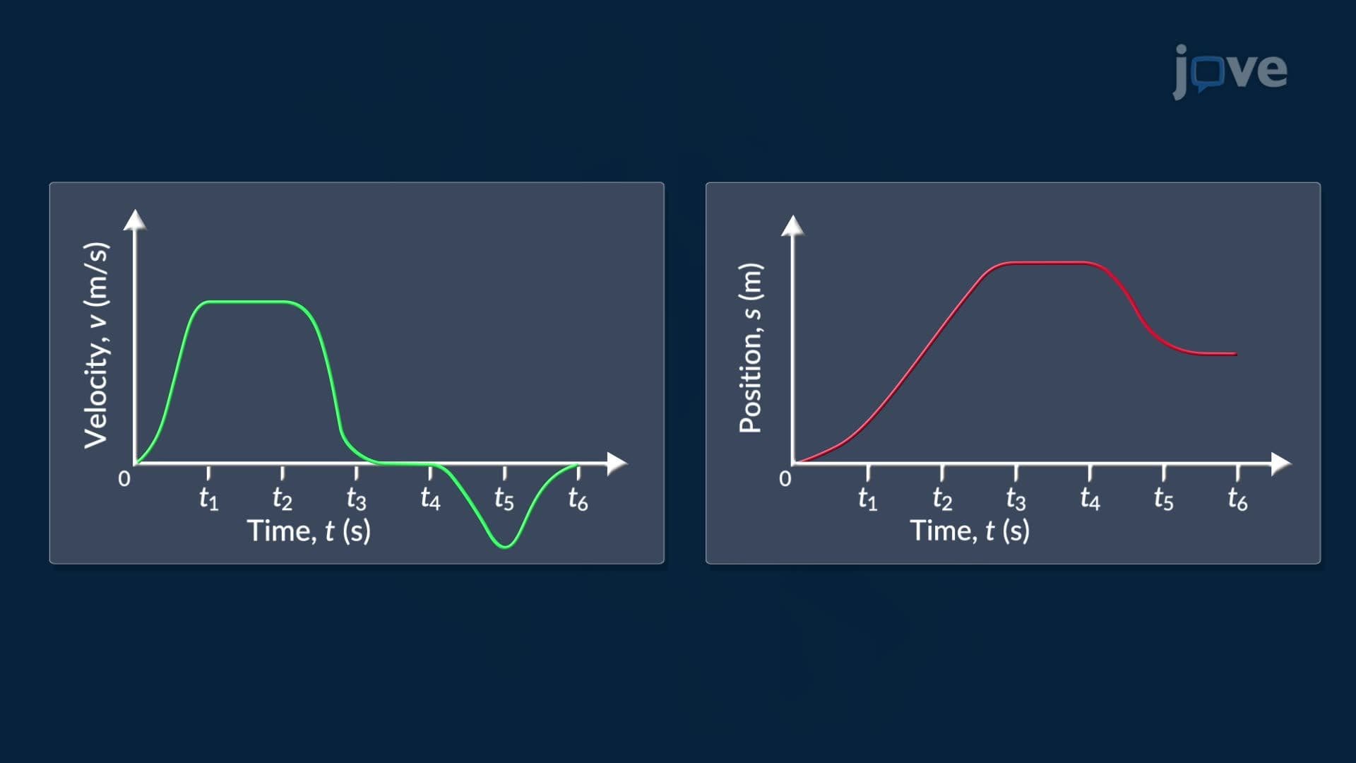
One of the clearest real-world applications of the antiderivative of a function explained is in kinematics, the study of motion. Suppose a physics student knows that a projectile's velocity function is v(t) = −32t + 60 (in feet per second). To find where the object is at any given moment, the student must find the antiderivative of v(t), which yields the position function s(t) = −16t² + 60t + C. The constant C is then determined using an initial condition, such as the starting height of the object. This same logic is used by engineers at organizations like SpaceX and NASA to model spacecraft trajectories when sensor data provides velocity readings rather than direct position measurements.
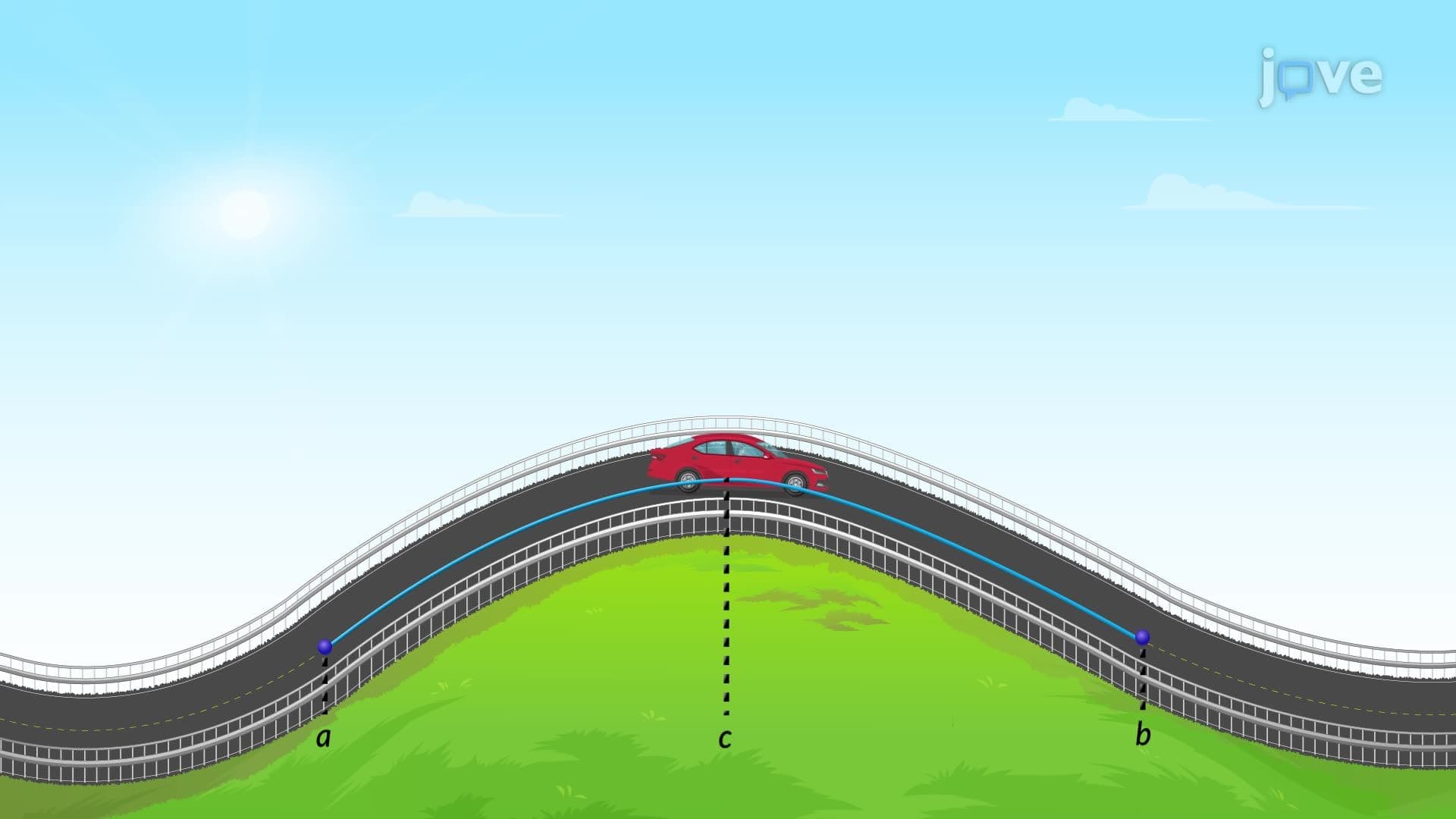
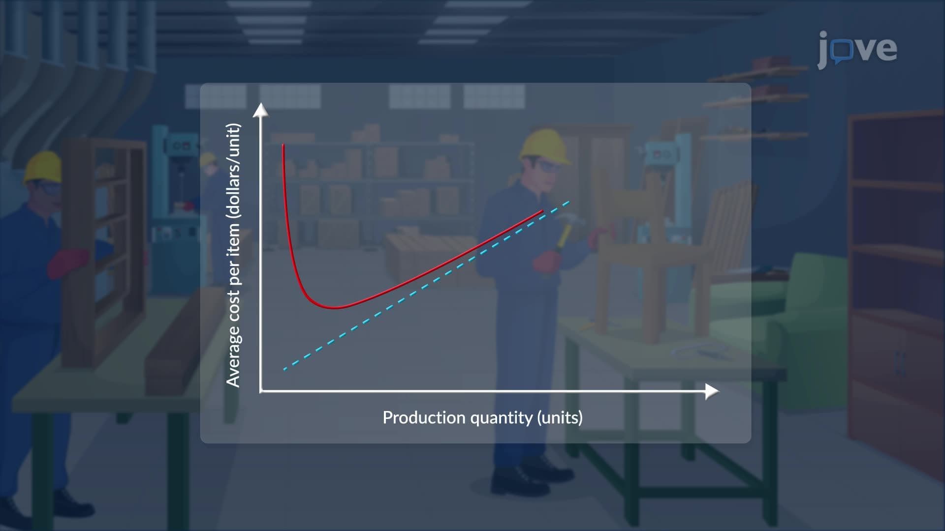
Mastering antiderivatives opens the door to a wide range of calculus topics tested on AP exams and college midterms. The relationship between a function and its antiderivative is directly tied to curve sketching, understanding whether a function is increasing or decreasing helps identify what its antiderivative looks like graphically. Concepts like concavity, inflection points, and maximum and minimum values all depend on moving fluidly between a function and its derivatives or antiderivatives. The Mean Value Theorem also relies on this relationship, as does the setup for optimization problems in which rates of change must be integrated to find total quantities. Even related rates problems, a staple of AP Calculus, become more tractable once students are comfortable reversing the differentiation process. Building a solid foundation in antiderivatives is not just about passing a test; it is the essential first step toward understanding the Fundamental Theorem of Calculus, definite integrals, and applied mathematical modeling.
Related Micro-courses