Loading video…

 19 Concepts
 5.7K views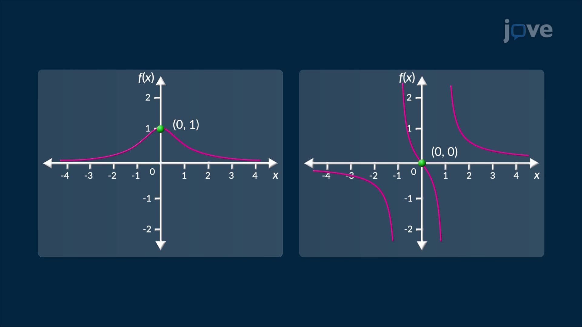

Video Summary: Guidelines for Sketching a Curve Explained
Ever wonder why roller coasters curve so perfectly, or how biologists model population explosions? Understanding the guidelines for sketching a curve unlocks the math behind these real-world shapes. This concept, guidelines for sketching a curve basics, walks you through domain, intercepts, symmetry, asymptotes, and derivative analysis. A classic US example: the logistic growth model used in ecology courses at universities like Stanford. Watch the full video on JoVE Coach to master this concept with expert-led visuals and step-by-step explanations.
Curve sketching is one of the most powerful skills in calculus because it turns abstract equations into visual stories. Rather than just plotting random points, the guidelines for sketching a curve give students a structured checklist that reveals everything meaningful about a function's behavior, where it lives, how it moves, and where it turns. Mastering this process is central to AP Calculus AB and BC, college calculus courses, and even standardized tests like the SAT Subject Math Level 2.
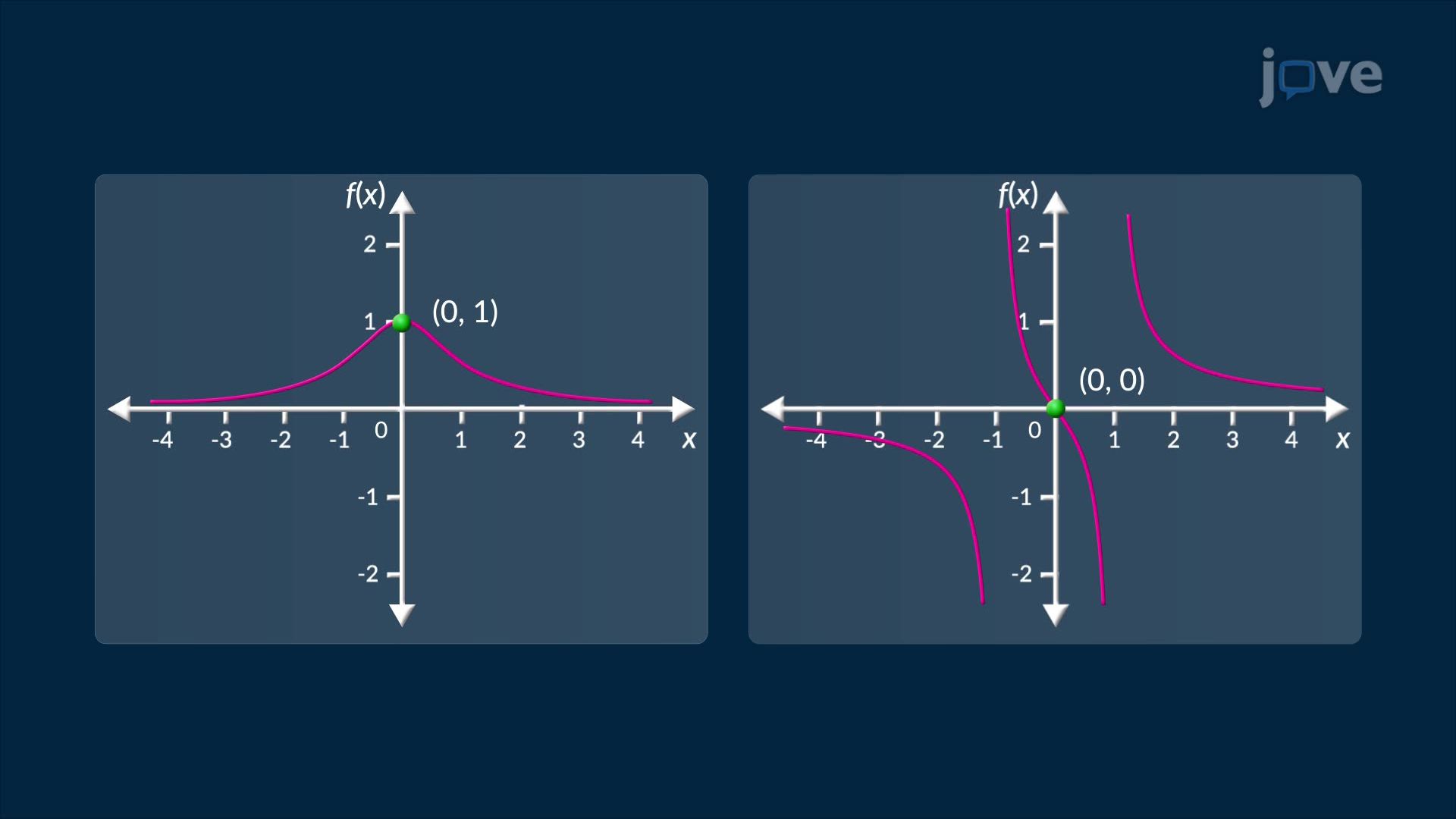
Every curve sketch begins with the basics. The domain identifies all valid input values, essentially, where the function "exists" on the horizontal axis. For example, a rational function like f(x) = 1/(x − 2) has a domain of all real numbers except x = 2. Next, intercepts, where the curve crosses the axes, act as anchor points for the sketch. Setting f(x) = 0 finds x-intercepts; setting x = 0 finds y-intercepts. Finally, checking for symmetry (even functions symmetric about the y-axis, odd functions symmetric about the origin) can cut your work in half, a useful time-saver during AP exam free-response sections.
Asymptotes act like invisible rails guiding a curve's overall shape. Vertical asymptotes occur where the function approaches infinity, typically where the denominator equals zero. Horizontal asymptotes emerge by evaluating the limit of f(x) as x approaches positive or negative infinity, a direct application of limit theory taught in every US college calculus course. Understanding asymptotic behavior is essential for optimization problems and related rates problems, where knowing a function's boundaries prevents costly errors in interpretation.
The first derivative, f'(x), measures the slope of the tangent line at any point. Setting f'(x) = 0 or finding where it is undefined reveals critical points, locations where the function may reach a local maximum or minimum. Applying the first derivative test means checking whether f'(x) changes sign around each critical point. If f'(x) goes from positive to negative, the function has a local maximum; negative to positive signals a local minimum. This directly supports solving maximum and minimum values problems, which appear frequently on AP Calculus exams and college midterms across the United States.
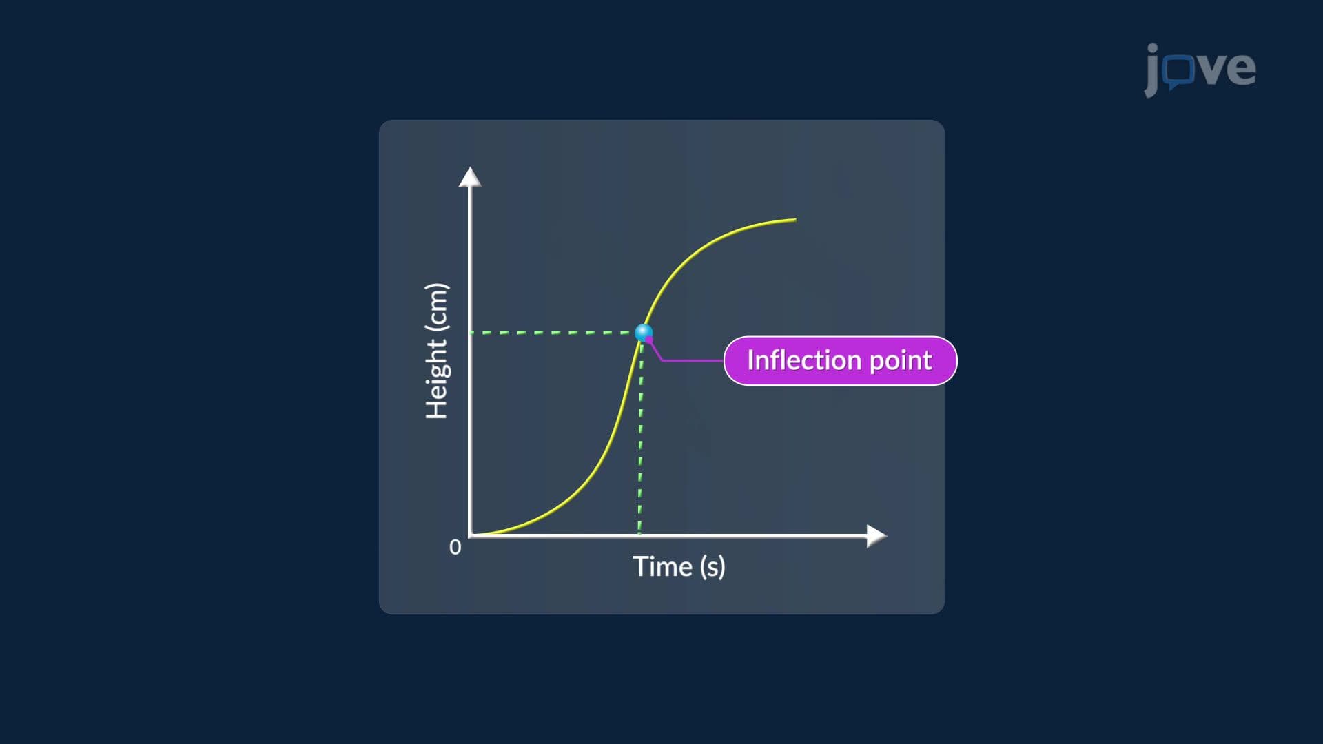
The second derivative, f''(x), reveals the curve's concavity, whether it bends upward (concave up, like a bowl) or downward (concave down, like a hill). Where f''(x) changes sign, an inflection point exists, a location where curvature reverses direction. A compelling real-world example is the logistic growth model, used extensively in US biology and ecology courses. The S-shaped logistic curve features a horizontal asymptote representing maximum population capacity and a single inflection point marking where growth rate transitions from accelerating to decelerating. This model appears in AP Biology, AP Environmental Science, and introductory college ecology courses nationwide. Together, all four steps create a complete, accurate, and mathematically justified sketch, far more reliable than guesswork alone.
Related Micro-courses