Loading video…

 17 Concepts
 6.3K views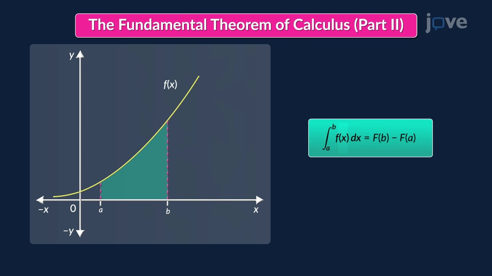

Video Summary: Fundamental Theorem of Calculus Ii Explained
Ever wonder how engineers at NASA calculate the exact distance a rocket travels during a burn without tracking every millisecond? The answer lies in the Fundamental Theorem of Calculus II. This powerful theorem connects antiderivatives to definite integrals, letting you compute precise accumulations over any interval, no estimation required. A classic US classroom example: finding a car's net displacement from its velocity function. Watch the full video on JoVE Coach to master this concept with expert-led visuals and step-by-step explanations.
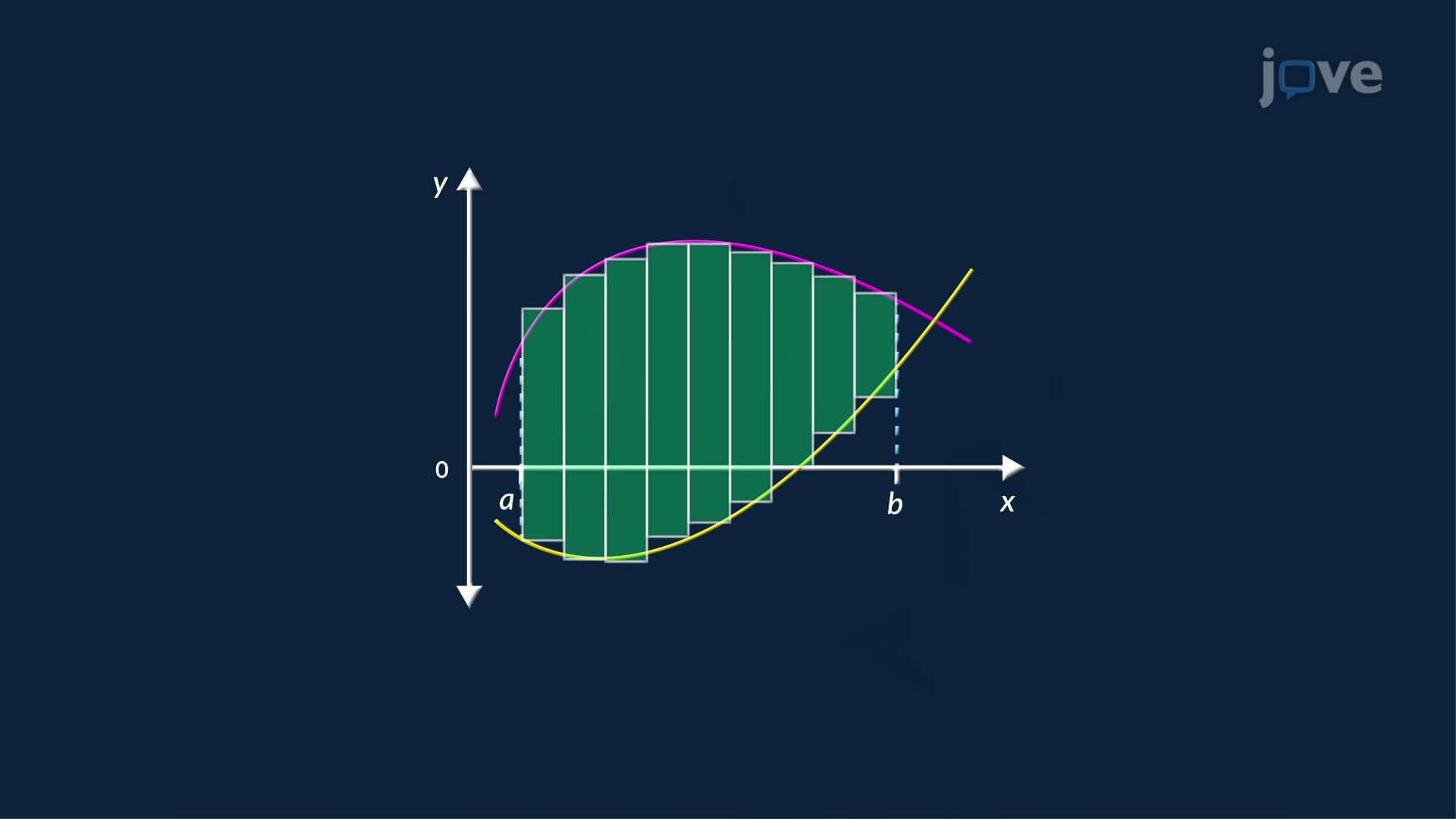
The Fundamental Theorem of Calculus II (FTC II) is one of the most important results in all of mathematics. It establishes a direct, clean connection between two ideas that might seem unrelated at first glance: the antiderivative of a function and the definite integral over an interval. Before this theorem, computing exact areas under curves required Riemann sums, a process of slicing a region into hundreds of narrow rectangles and adding their areas. FTC II eliminates that tedious approximation entirely. If you can find an antiderivative, you can compute the exact value of any definite integral.
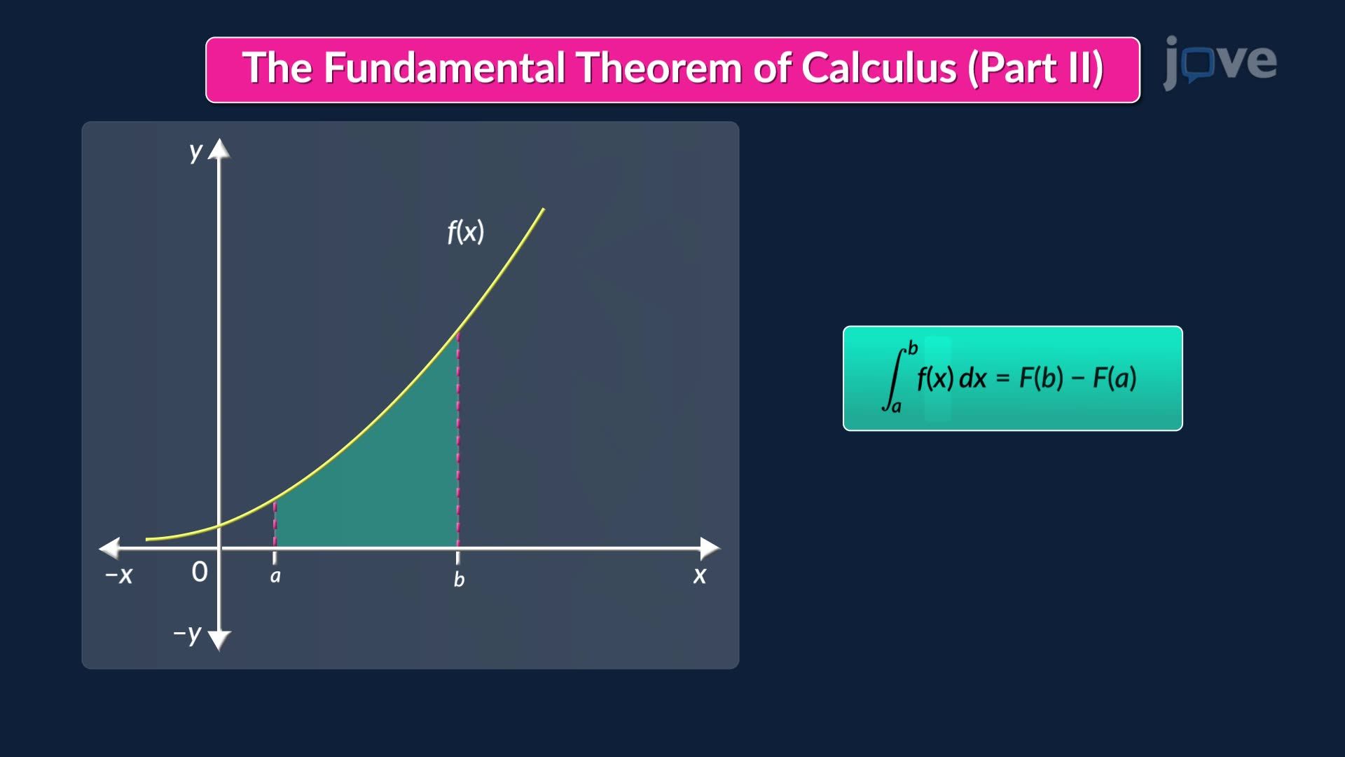
Formally stated: if a function f(x) is continuous on a closed interval [a, b], and F(x) is any antiderivative of f(x), then the definite integral of f from a to b equals F(b) minus F(a). In plain notation: ∫(a to b) f(x) dx = F(b) − F(a). This deceptively simple formula is the engine behind a massive range of calculations in physics, economics, biology, and engineering.
A common source of confusion is the difference between definite and indefinite integrals. An indefinite integral produces a family of antiderivatives, it outputs a function plus a constant C, because infinitely many antiderivatives differ only by a vertical shift. A definite integral, by contrast, produces a single numerical value. It represents the net accumulation of a quantity over a specific interval. FTC II is precisely the bridge between them: it uses the indefinite integral (the antiderivative) as a tool to evaluate the definite integral. Critically, the constant C always cancels during subtraction, [F(b) + C] − [F(a) + C] = F(b) − F(a), so your choice of antiderivative never affects the final answer.
Evaluating a definite integral with FTC II follows a consistent three-step process:
1. Find the antiderivative of the integrand. For example, if f(x) = 3x², the antiderivative is F(x) = x³. 2. Substitute the upper and lower limits into F(x). Compute F(b) and F(a) separately. 3. Subtract: F(b) − F(a) gives the exact value of the definite integral.
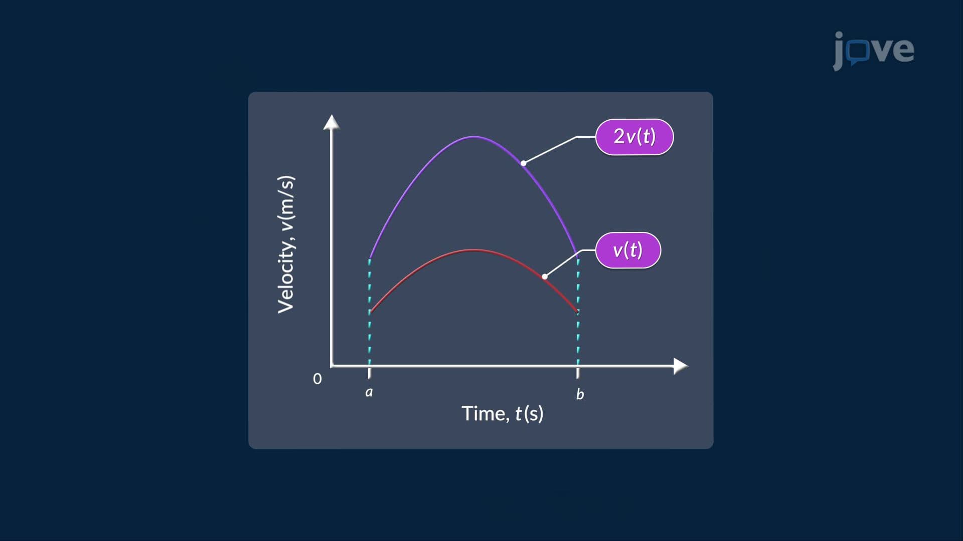
For a US classroom-style example: suppose a car's velocity is given by v(t) = 3t² feet per second. To find the net displacement from t = 1 to t = 4 seconds, integrate v(t) from 1 to 4. The antiderivative is F(t) = t³. Evaluating: F(4) − F(1) = 64 − 1 = 63 feet. No Riemann sum needed, one clean calculation gives the exact answer. This type of problem appears regularly on the AP Calculus AB and BC exams, as well as college Calculus I midterms across the US.
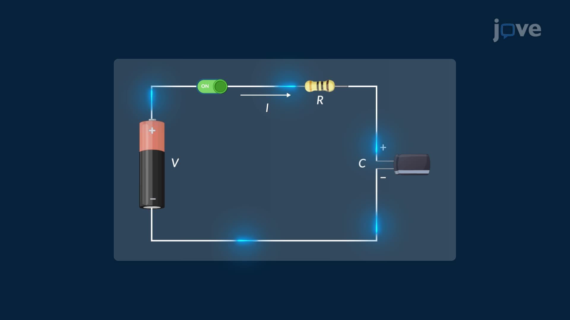
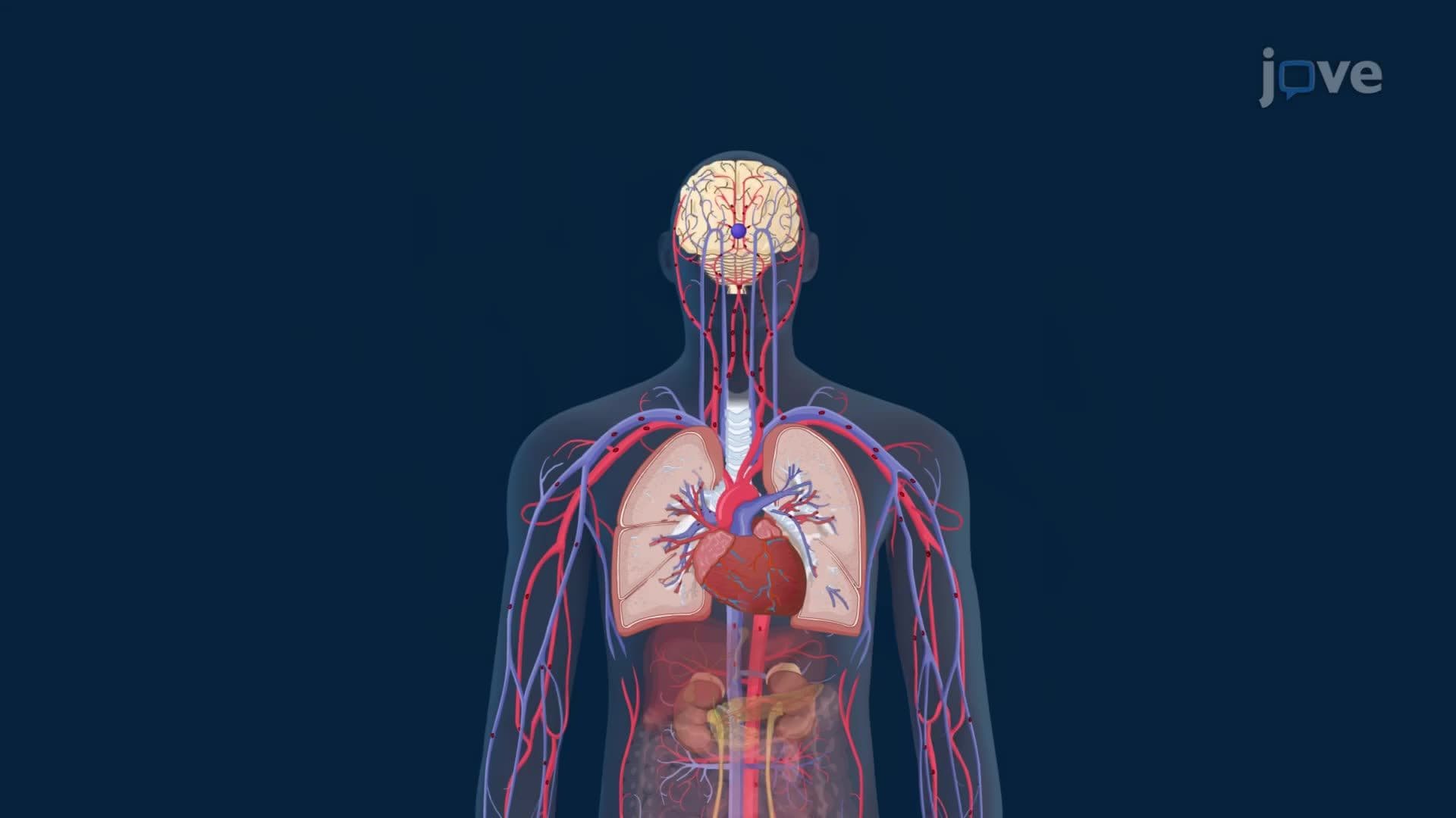
The Fundamental Theorem of Calculus II shows up far beyond the classroom. In physics, it calculates work done by a variable force, a standard topic in AP Physics C. In economics, it finds total revenue accumulated over time given a marginal revenue function. In medicine and biology, it models the total drug concentration absorbed by the body over a dosing interval, a concept relevant to pharmacokinetics covered in pre-med and MCAT preparation.
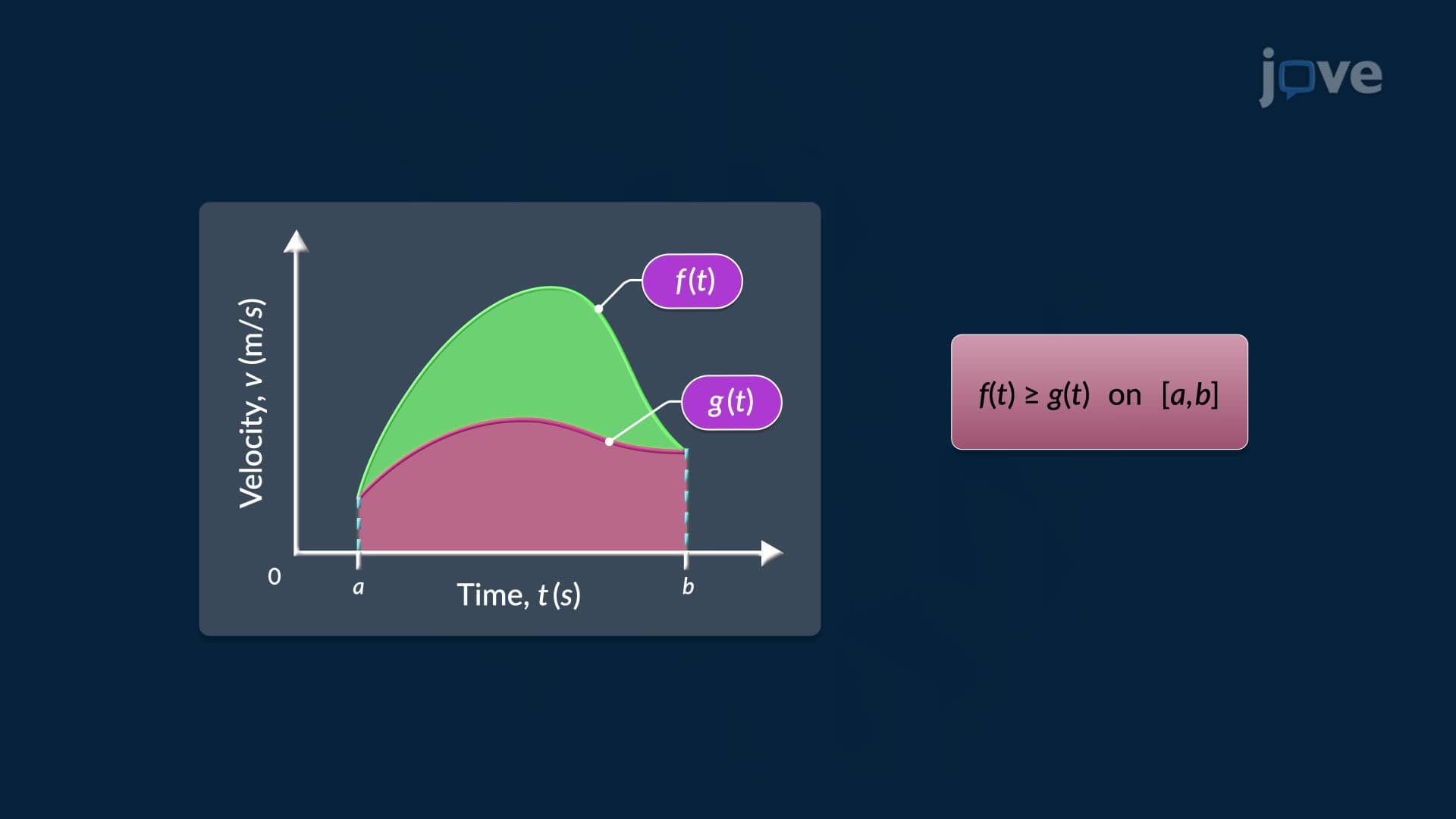
On the AP Calculus AB exam, FTC II is a guaranteed topic. Students are expected to set up definite integrals from context, apply the theorem procedurally, and interpret the result, often as displacement, total growth, or net change. Understanding the properties of integrals, including additivity over intervals and the behavior of even and odd functions, further strengthens exam performance and deepens conceptual fluency in college-level calculus.
Related Micro-courses