Loading video…

 17 Concepts
 6.3K views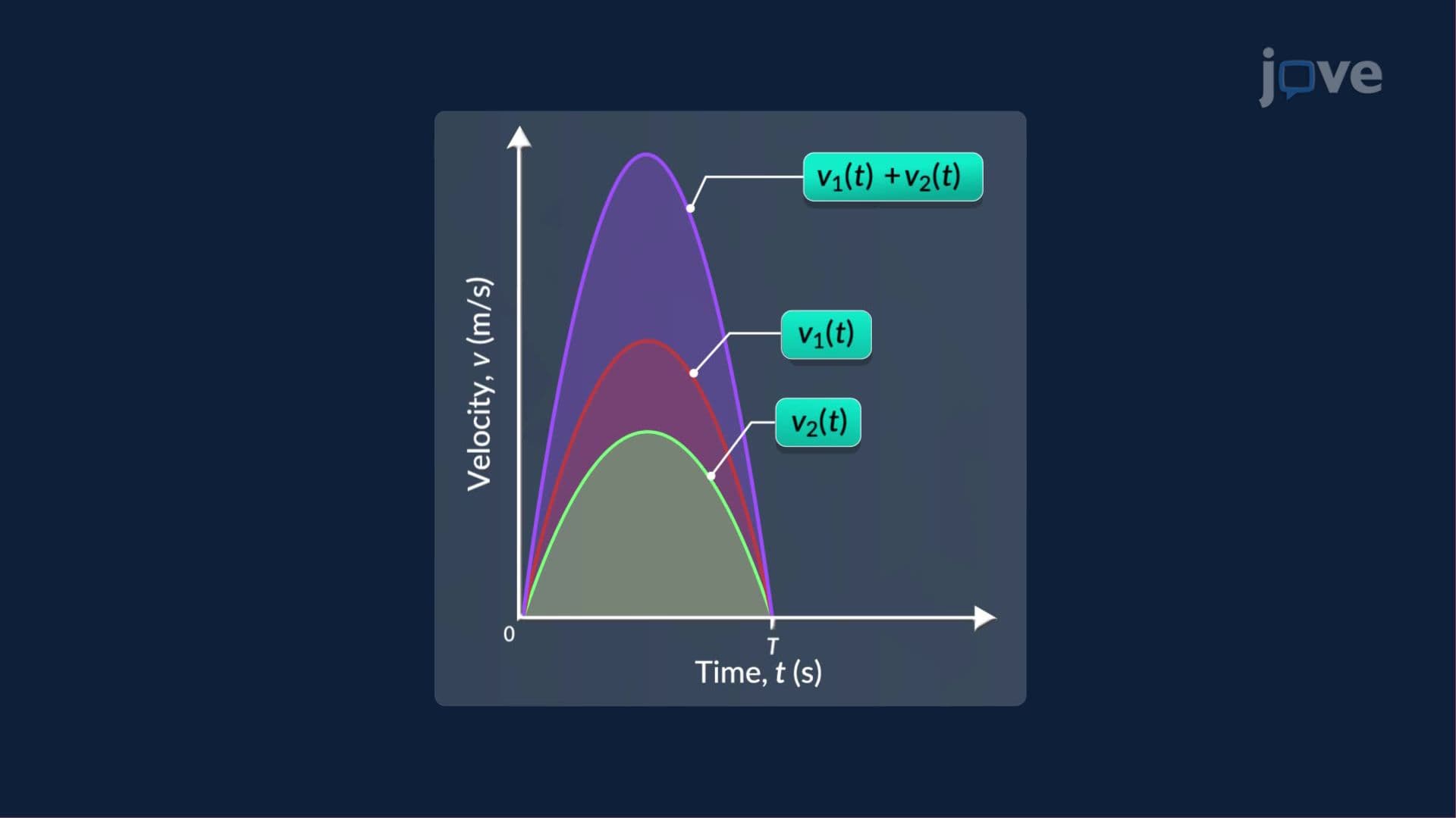

Video Summary: Properties of Definite Integral I Explained
Ever wonder how engineers at NASA calculate a rocket's total displacement when its velocity changes every second? The Properties of Definite Integral I, also called Properties of Definite Integral I basics, unlock powerful shortcuts for solving exactly these kinds of problems. Two foundational rules, linearity (addition and subtraction of integrals) and integrating constant functions, let you break complex motion problems into manageable pieces. Watch the full video on JoVE Coach to master this concept with expert-led visuals and step-by-step explanations.
The Properties of Definite Integral I are not just abstract rules, they are the logical scaffolding that makes integration practical and efficient. Before memorizing formulas, students benefit from understanding *why* these properties hold, grounding them in both geometry (area under a curve) and the algebraic structure of limits used in Riemann sums. Mastering these properties is essential for success in AP Calculus AB, AP Calculus BC, college Calculus I, and even standardized tests like the SAT Subject Tests and MCAT quantitative reasoning sections.
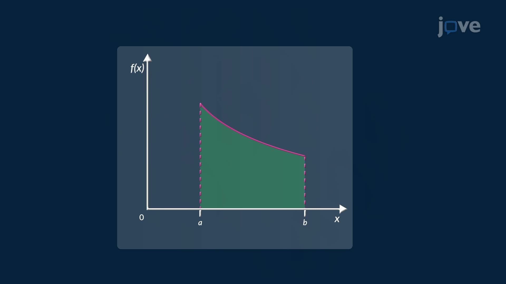
A definite integral computes the *net accumulation* of a quantity over a specific interval. Unlike indefinite integrals, which produce a family of antiderivatives (expressed with a constant C), definite integrals yield a single numerical value. For example, if a car on a California highway accelerates with a velocity described by v(t) = 3t² from t = 0 to t = 4 seconds, the definite integral of v(t) over that interval gives the exact displacement, no guessing required.
Understanding the difference between definite and indefinite integrals is a foundational concept tested repeatedly on the AP Calculus exam. The definite integral is bounded by two limits (a lower bound and an upper bound), while the indefinite integral is open-ended, representing all possible antiderivatives of a function.
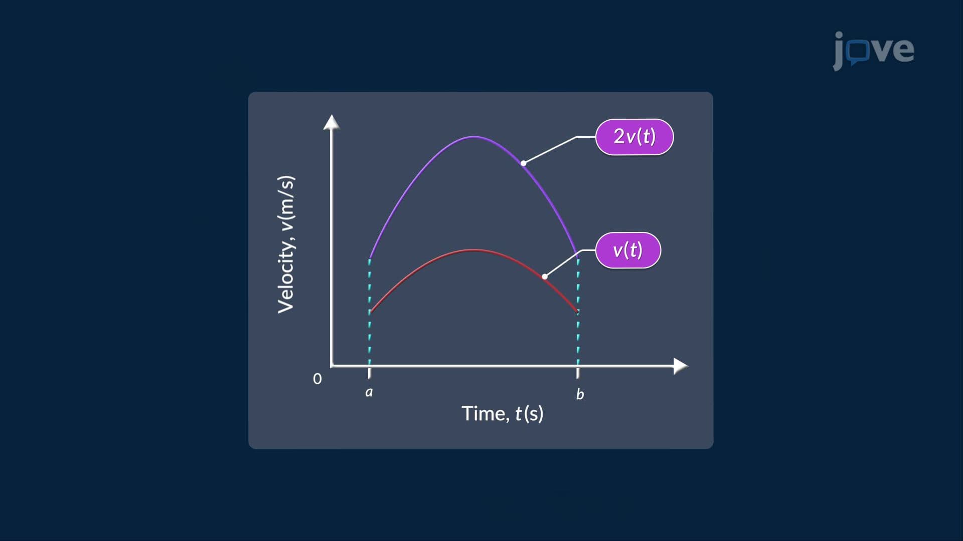
The linearity property is the most frequently applied rule among the Properties of Definite Integral I. It states two things:
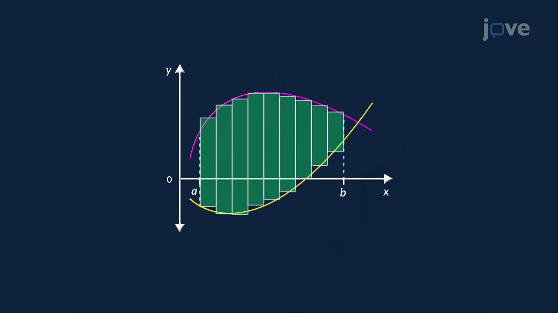
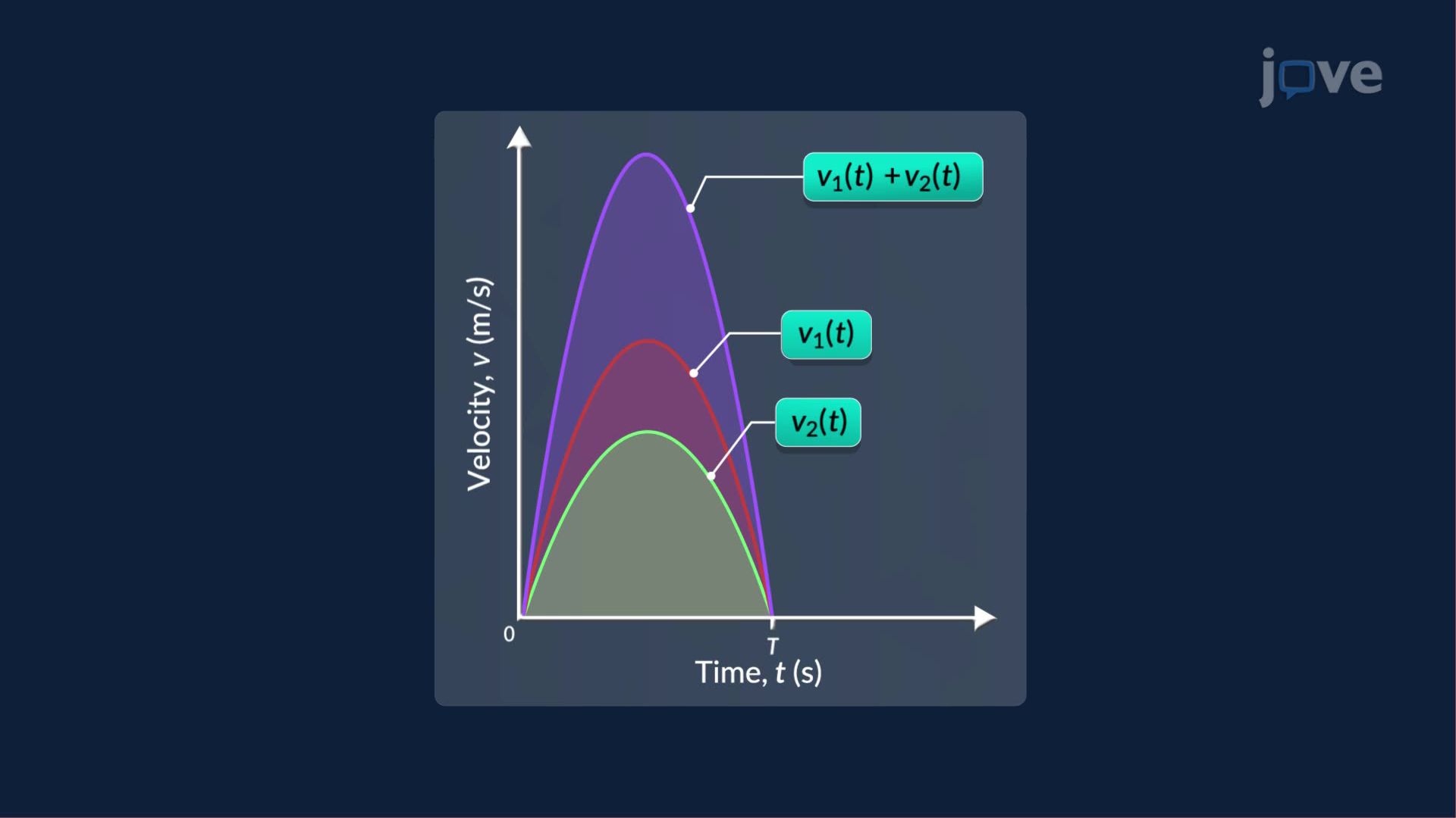
Geometrically, this makes perfect sense. If two separate road trips have velocity-time curves, the combined area under the summed curve is simply the total of the two individual areas. This property works because integration is defined as a limit of Riemann sums, and limits distribute across addition and subtraction.
In practice, this property lets students simplify otherwise unmanageable integrals. On the AP Calculus BC exam, multi-part free-response questions frequently require students to split integrals of combined functions, a direct application of linearity.
When a function's value does not change over an interval, like a car cruising at a steady 60 mph on an interstate, its integral is simply the constant multiplied by the length of the interval:
∫[a to b] c dx = c × (b − a)
This is geometrically equivalent to finding the area of a rectangle: base times height. While simple, this property is a critical checkpoint in evaluating piecewise functions and step functions, which appear frequently in college Calculus I courses and on AP exam multiple-choice sections.
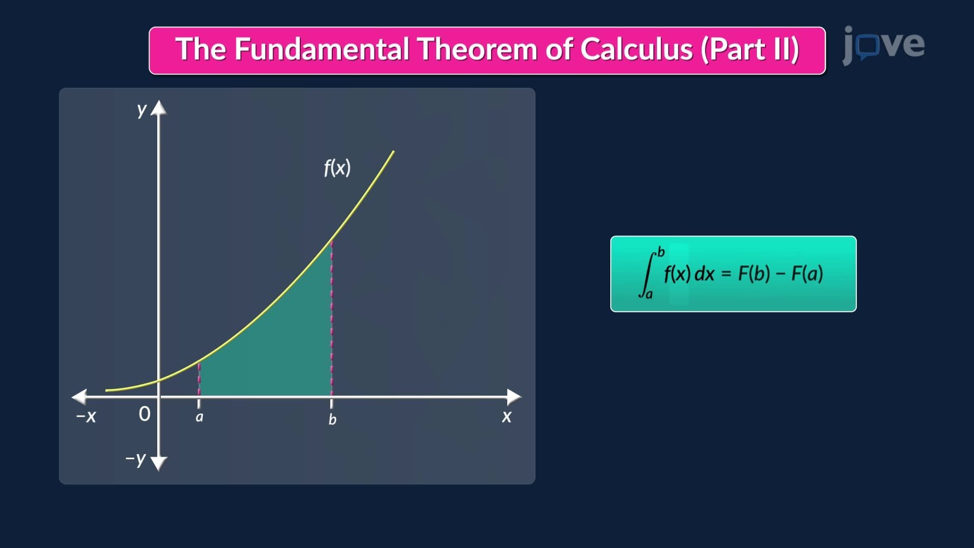
These properties work hand in hand with the Fundamental Theorem of Calculus, which links antiderivatives to definite integrals. Once students learn to evaluate ∫[a to b] f(x) dx as F(b) − F(a), where F is an antiderivative of f, the linearity and constant-function properties make breaking apart complex expressions far more manageable.
For AP Calculus students, a practical study strategy is to identify which property applies *before* attempting to compute. Recognizing a sum or a constant early saves time under exam pressure and reduces errors significantly.
Related Micro-courses