Indefinite Integrals

• Understand what indefinite integrals are and how they differ from simply evaluating a function at a single point in time
• Identify the relationship between antiderivatives and indefinite integrals, recognizing that integration reverses the process of differentiation
• Analyze how a linear rate function, when integrated, produces a quadratic volume function that captures accelerating growth
• Compare definite and indefinite integrals, distinguishing between finding a numeric area under a curve versus generating a general function with a constant of integration
• Apply indefinite integration to real-world rate problems, such as calculating fluid volume in an industrial tank given a time-varying inflow rate
• Recognize the role of the constant of integration (C) and how initial conditions — like the volume of water at time zero — are used to determine its value
• Evaluate how the Fundamental Theorem of Calculus connects antiderivatives to the broader framework of integral calculus
• Explore how properties of integrals — including linearity and scalar multiplication — simplify the integration of complex expressions

What Are Indefinite Integrals? Building Intuition from the Ground Up

An indefinite integral is the mathematical tool that answers this question: *if I know how fast something is changing, can I find the total amount accumulated over time?* In calculus, this is the process of antidifferentiation — working backward from a rate of change to find the original quantity function. Unlike definite integrals, which return a specific numerical value over a fixed interval, indefinite integrals return a family of functions, each differing by a constant. That constant — written as *C* — is the constant of integration, and it accounts for any initial condition baked into the problem.

Antiderivatives: The Engine Behind Indefinite Integration

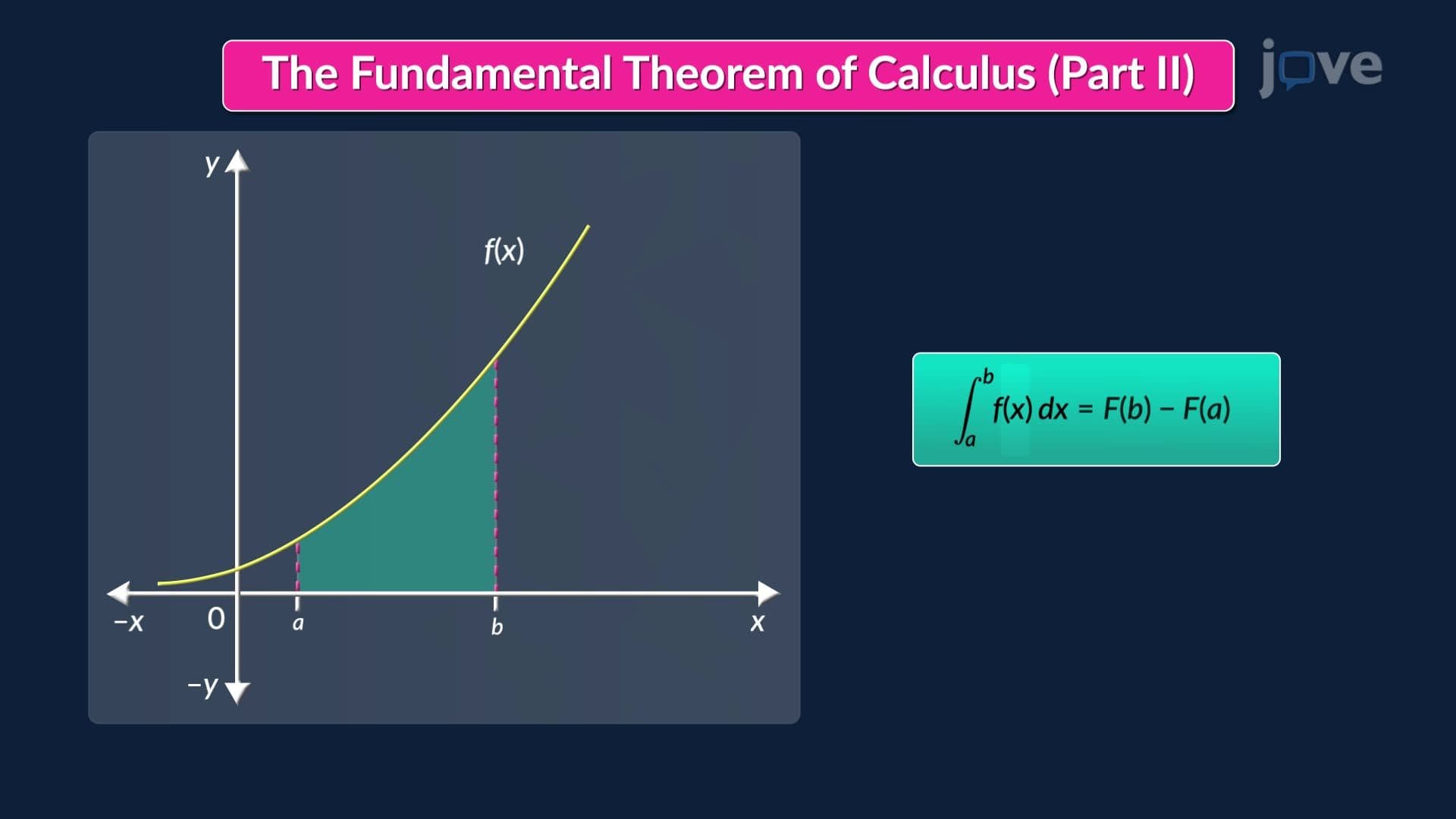
At the heart of indefinite integrals is the concept of an antiderivative. If F(x) is a function whose derivative is f(x), then F(x) is called the antiderivative of f(x), and the indefinite integral of f(x) is written as ∫f(x) dx = F(x) + C. For example, the antiderivative of 2x is x² + C, because differentiating x² gives 2x. This reverse relationship is formalized by the Fundamental Theorem of Calculus, which bridges differentiation and integration — one of the most powerful ideas in all of mathematics and a guaranteed topic in AP Calculus AB and BC.

Definite and Indefinite Integrals: What's the Difference?

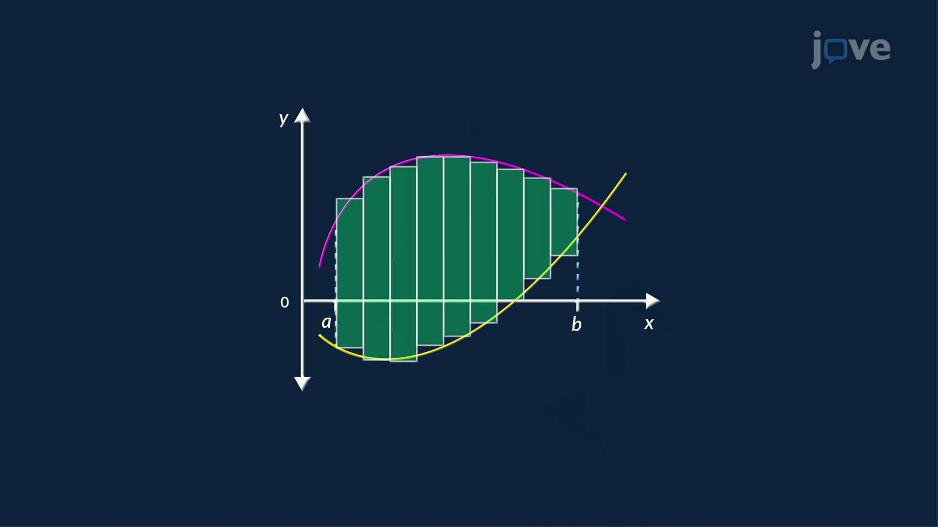
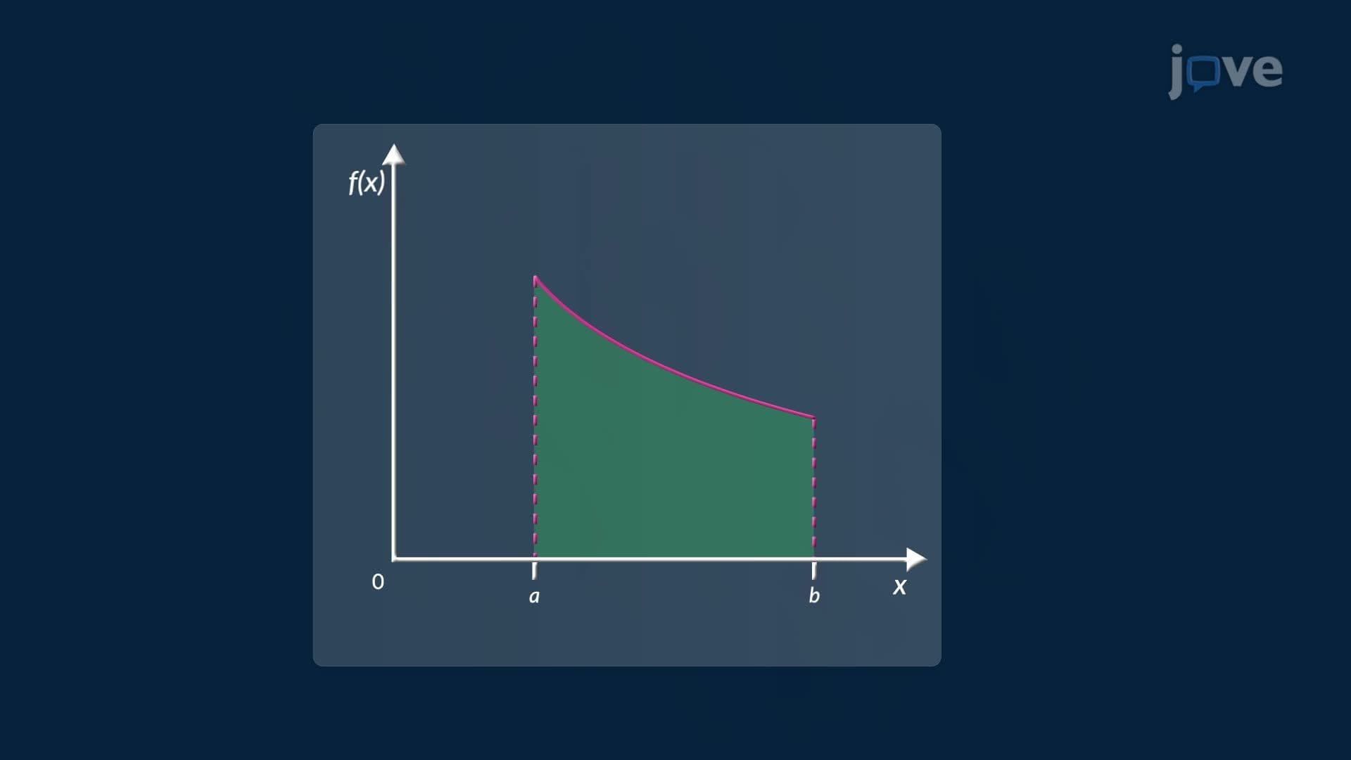
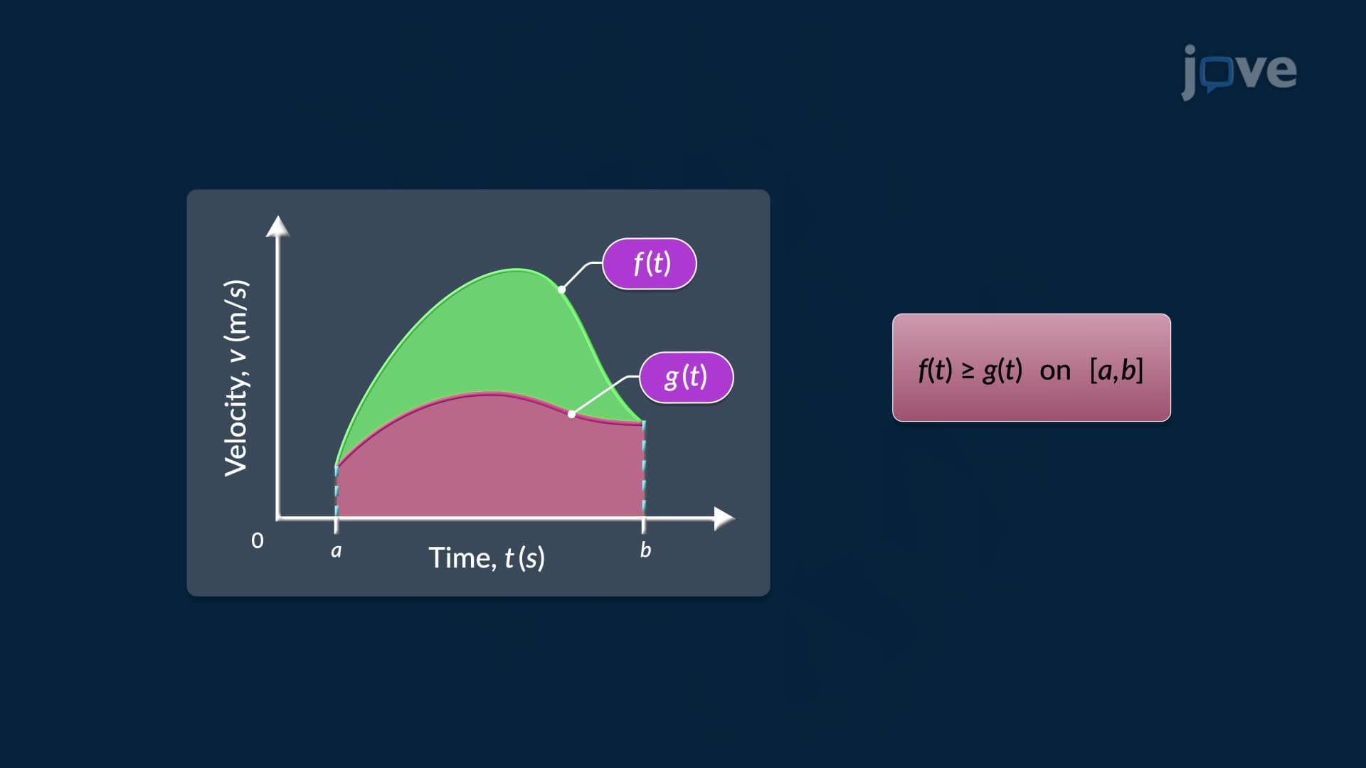
Students often confuse these two types. A definite integral has upper and lower limits of integration and produces a single number — typically representing an area under a curve or net change over an interval. An indefinite integral has no bounds; it produces a general function. Think of it this way: if a definite integral tells you how much water filled a tank *between hour 1 and hour 3*, an indefinite integral gives you the formula to find the volume *at any time*. On AP Calculus exams and college midterms, questions often test whether students correctly attach the constant *C* to indefinite results — a common and costly oversight.

Real-World Applications and How to Calculate Integrals

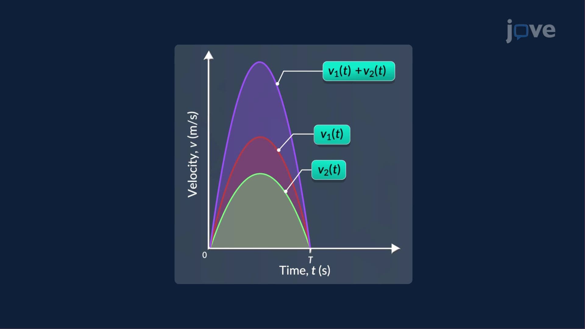
Indefinite integrals appear everywhere in science and engineering. In physics, integrating acceleration gives velocity; integrating velocity gives position. In environmental science, US agencies like the EPA model pollutant accumulation by integrating time-varying emission rates. In economics, integrating a marginal cost function recovers the total cost function. Knowing how to calculate integrals starts with mastering basic rules: the Power Rule (∫x^n dx = x^(n+1)/(n+1) + C), the Constant Multiple Rule, and the Sum Rule. These properties of integrals allow complex expressions to be broken into manageable pieces. For students preparing for AP Calculus, STEM college courses, or even the math section of standardized tests, fluency with these integration rules is non-negotiable. Practice by starting with polynomial functions — like the linear inflow rate example — and build toward trigonometric and exponential integrals as confidence grows.