Loading video…

 17 Concepts
 6.3K views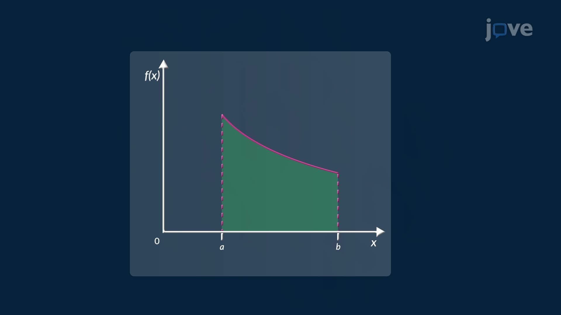

Video Summary: What Is Midpoint Rule
Estimating the area under a curve sounds complex, but what if rectangles could do the job? The midpoint rule is a foundational technique in calculus that approximates this area by splitting an interval into equal subintervals and using each midpoint as the rectangle's height. Engineers at the US Army Corps of Engineers use similar methods to estimate riverbank areas for flood planning. What is Midpoint Rule? It's your first step toward understanding definite integrals. Watch the full video on JoVE Coach to master this concept with expert-led visuals and step-by-step explanations.
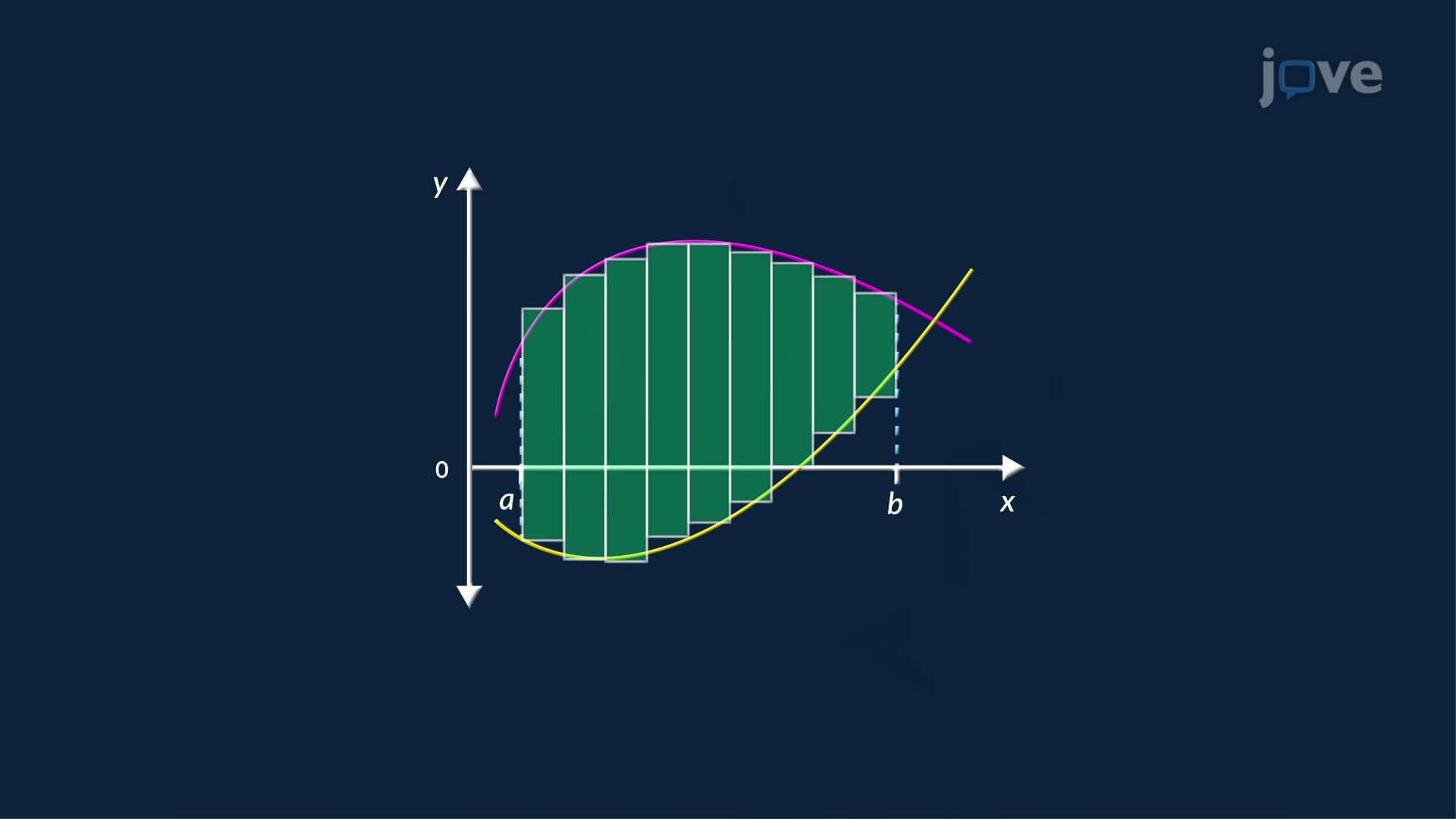
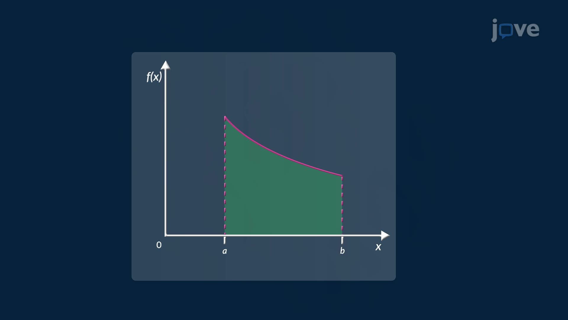
The Midpoint Rule is a numerical integration technique that estimates the area under a curve by dividing a given interval into *n* equal subintervals and constructing a rectangle over each one. Unlike guessing at the height using the left or right edge of each subinterval, the Midpoint Rule samples the function at the center point of each subinterval. This single adjustment dramatically reduces the overestimation and underestimation errors that plague left- and right-endpoint methods, making it one of the most accessible and accurate entry-level approximation strategies in calculus.
To apply the Midpoint Rule over an interval [a, b] with *n* subintervals, follow these steps:
1. Calculate subinterval width: Δx = (b − a) / n 2. Find each midpoint: For the *i*-th subinterval, the midpoint is m(i) = a + (i − 0.5) × Δx 3. Evaluate the function at each midpoint: f(m(1)), f(m(2)), … f(m(n)) 4. Apply the formula: Midpoint Rule ≈ Δx × [f(m(1)) + f(m(2)) + … + f(m(n))]
This summation is a specific type of Riemann sum, a concept that bridges the gap between discrete rectangle approximations and the exact value of a definite integral. As *n* increases toward infinity, the Midpoint Rule approximation converges to the true area, which is expressed formally through the definite integral.
In AP Calculus AB and BC, students regularly compare three primary Riemann sum approaches: left-endpoint, right-endpoint, and midpoint. For a function that is concave up (like a U-shape), the left and right endpoint methods either overestimate or underestimate the area, while the Midpoint Rule actually underestimates, but by a far smaller margin. For concave down curves, the pattern reverses. Understanding this behavior is critical for AP free-response questions, where students are asked to determine whether an approximation is an overestimate or underestimate and justify their reasoning.
The Midpoint Rule also serves as a conceptual stepping stone toward the Trapezoidal Rule and Simpson's Rule, two more refined approximation methods introduced in AP Calculus BC and college-level Calculus II courses.
The Midpoint Rule isn't just a classroom exercise. Environmental engineers in the US use numerical integration to estimate the volume of water flowing through irregular stream cross-sections, where no clean algebraic formula describes the boundary. Similarly, NASA mission planners use numerical methods, rooted in the same principles, to approximate trajectories when exact solutions are computationally expensive.
On the AP Calculus AB exam, the Midpoint Rule frequently appears in both multiple-choice and free-response sections under the topic of "approximating areas." Students are typically given a table of function values and asked to apply the Midpoint Rule directly, no antiderivatives required. This makes it an essential skill for students who want to earn full credit on approximation problems without needing to evaluate a definite integral analytically.
In college Calculus I and II courses, the Midpoint Rule reinforces the conceptual meaning of the definite integral before students tackle antiderivatives and the Fundamental Theorem of Calculus. Grasping this approximation method first makes the transition to exact integration far more intuitive.
Related Micro-courses