Loading video…


 17 Concepts
 6.3K views

Video Summary: What Is Definite Integral
How do you calculate the exact area beneath a curved line, something no simple ruler can measure? That's exactly what the definite integral solves. Definite integral basics begin with Riemann sums, where a curve is approximated using stacked rectangles that get infinitely thin. A real-world US example: calculating the distance a car travels when its speed varies over time. Watch the full video on JoVE Coach to master this concept with expert-led visuals and step-by-step explanations.
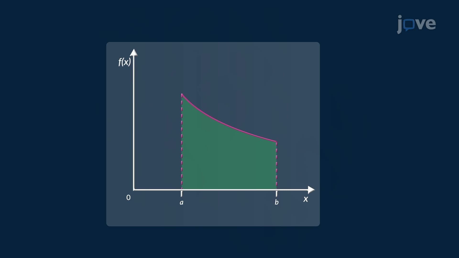
The definite integral is one of the most powerful tools in calculus. At its core, it answers a deceptively simple question: what is the exact area between a curve and the x-axis over a specific interval? While that might sound purely geometric, the concept drives real analysis in physics, economics, engineering, and medicine across the United States and beyond.
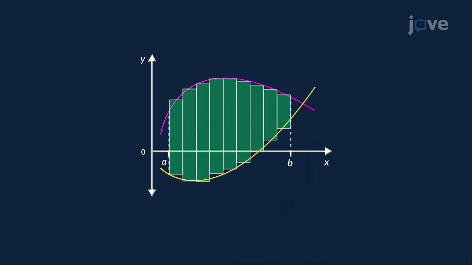
Before you can fully grasp the definite integral, you need to understand Riemann sums, the approximation method that gives it meaning. Imagine dividing the interval from point A to point B on the x-axis into *n* equal subintervals, each with width Δx = (B − A) / n. Inside each subinterval, you pick any point and evaluate the function there to get a rectangle's height. Multiply height by width, add up all the rectangles, and you have a Riemann sum.
The definite integral is defined as the limit of that Riemann sum as *n* approaches infinity, meaning the rectangles become infinitely narrow and the approximation becomes exact. Written formally, this is expressed as the integral from A to B of f(x) dx, where A and B are called the lower and upper limits of integration. When this limit exists, the function is said to be integrable on that interval.
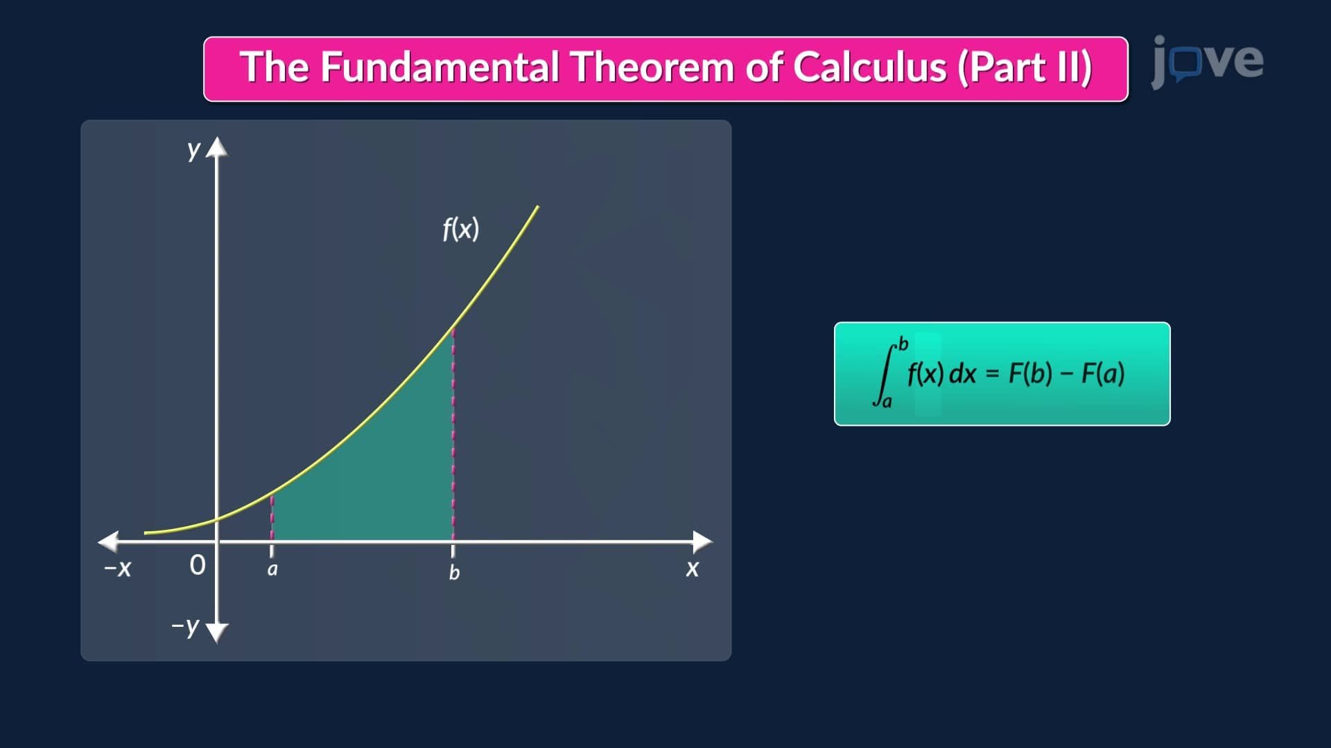
The Fundamental Theorem of Calculus is what makes definite integrals practically computable. It establishes that integration and differentiation are inverse operations. Specifically, if F(x) is an antiderivative of f(x), meaning F'(x) = f(x), then the definite integral from A to B of f(x) dx equals F(B) − F(A).
This theorem eliminates the need to compute Riemann sums by hand. For example, to find the area under the curve f(x) = 3x² from x = 1 to x = 4, you find the antiderivative F(x) = x³, then calculate F(4) − F(1) = 64 − 1 = 63. That's the exact area, solved in seconds.
Students often confuse definite and indefinite integrals, but they serve different purposes. An indefinite integral produces a general family of antiderivatives written as F(x) + C, where C is an arbitrary constant. There are no limits of integration, and the result is a function, not a number.
A definite integral, by contrast, always has upper and lower limits and produces a specific numerical value. Think of it this way: the indefinite integral tells you the shape of the antiderivative family, while the definite integral uses that family to measure something concrete, area, displacement, accumulated change.
In the US, definite integrals appear throughout AP Calculus AB and BC, college Calculus I and II courses, and even on the MCAT in physics-related passages. A classic application: if a car accelerates along a highway with velocity v(t) = 2t + 5 (in mph), the total distance traveled from t = 0 to t = 3 hours is found by evaluating the definite integral of v(t) over that interval.
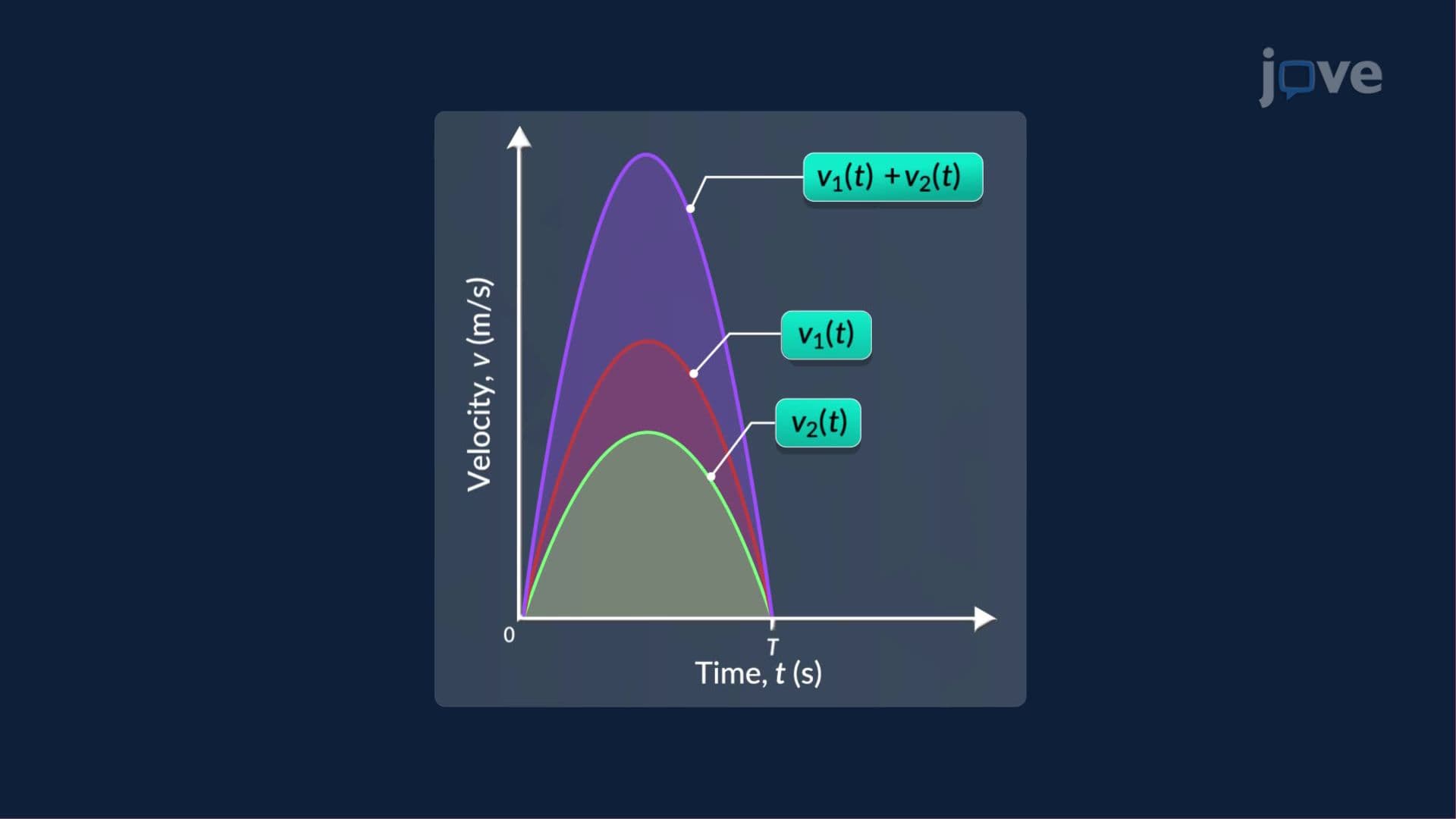
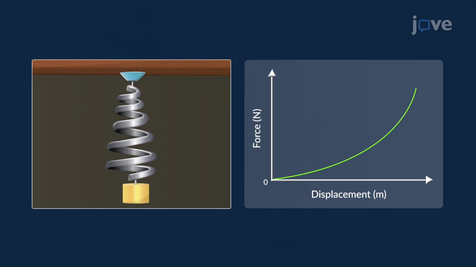
Beyond transportation, definite integrals model consumer surplus in economics, work done by a variable force in physics, and drug concentration over time in pharmacology, all topics covered in US undergraduate programs. Mastering the properties of integrals, such as splitting an integral over subintervals, reversing limits, and factoring out constants, makes solving these problems significantly faster on timed exams.
Related Micro-courses