Loading video…

 17 Concepts
 6.3K views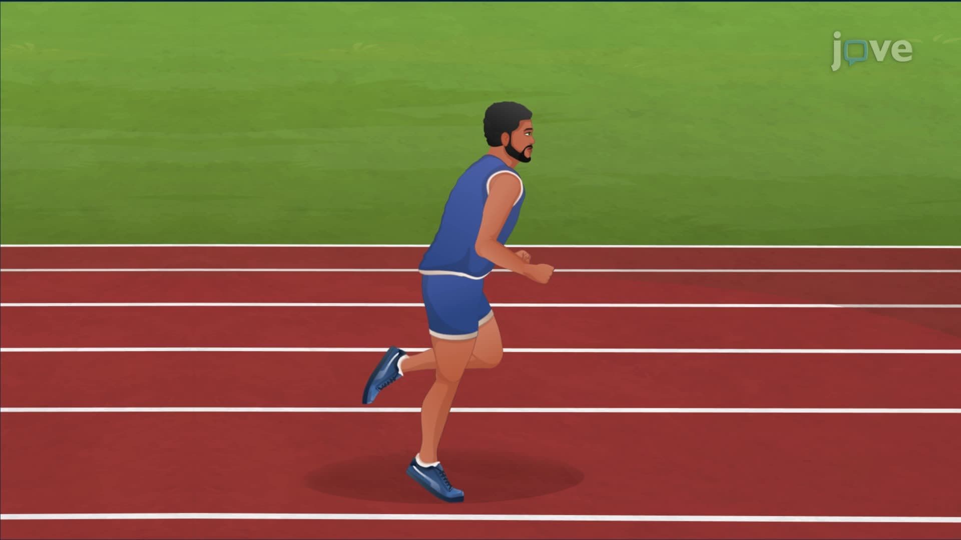

Video Summary: What Is Distance Problem
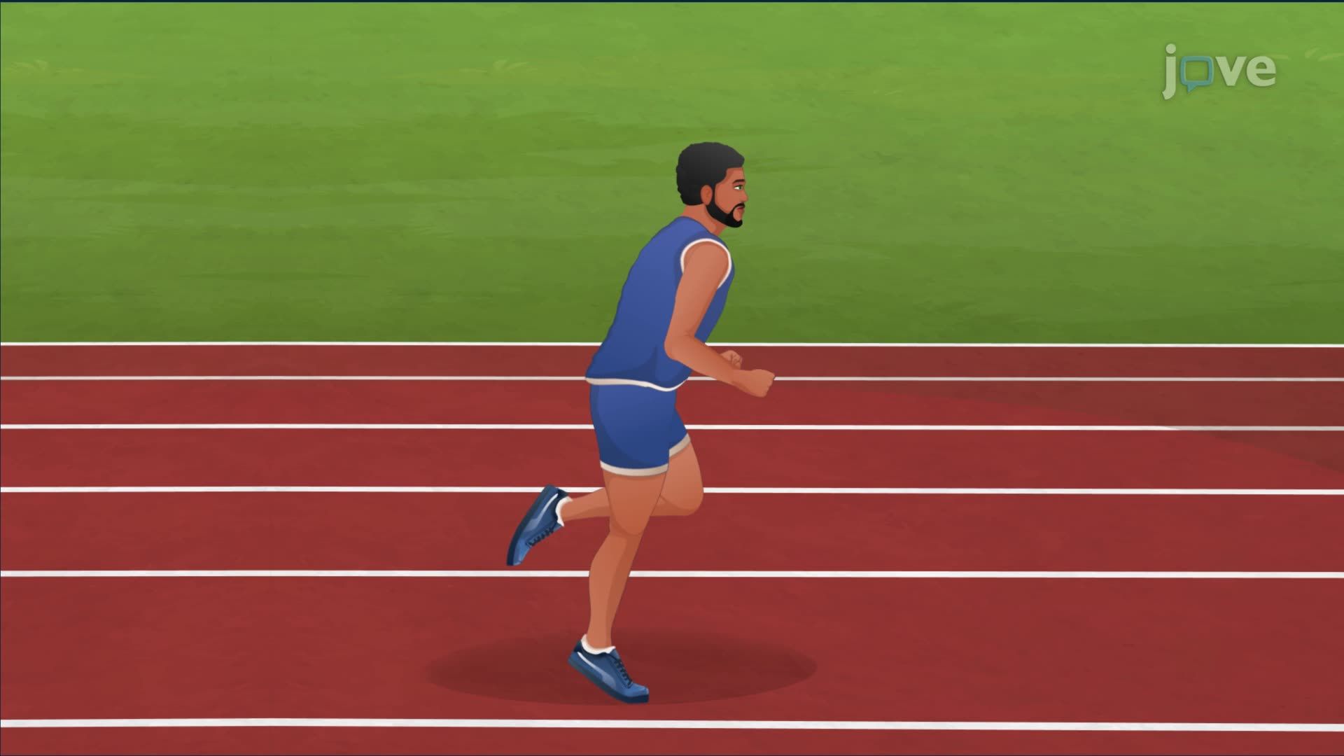
How far does a sprinter actually travel when their speed changes every second? The distance problem is a foundational calculus concept that estimates total distance traveled when velocity isn't constant. Using velocity data collected at timed intervals, much like GPS tracking in a US track-and-field event, the distance problem introduces Riemann sums and leads directly to definite integrals. Watch the full video on JoVE Coach to master this concept with expert-led visuals and step-by-step explanations.
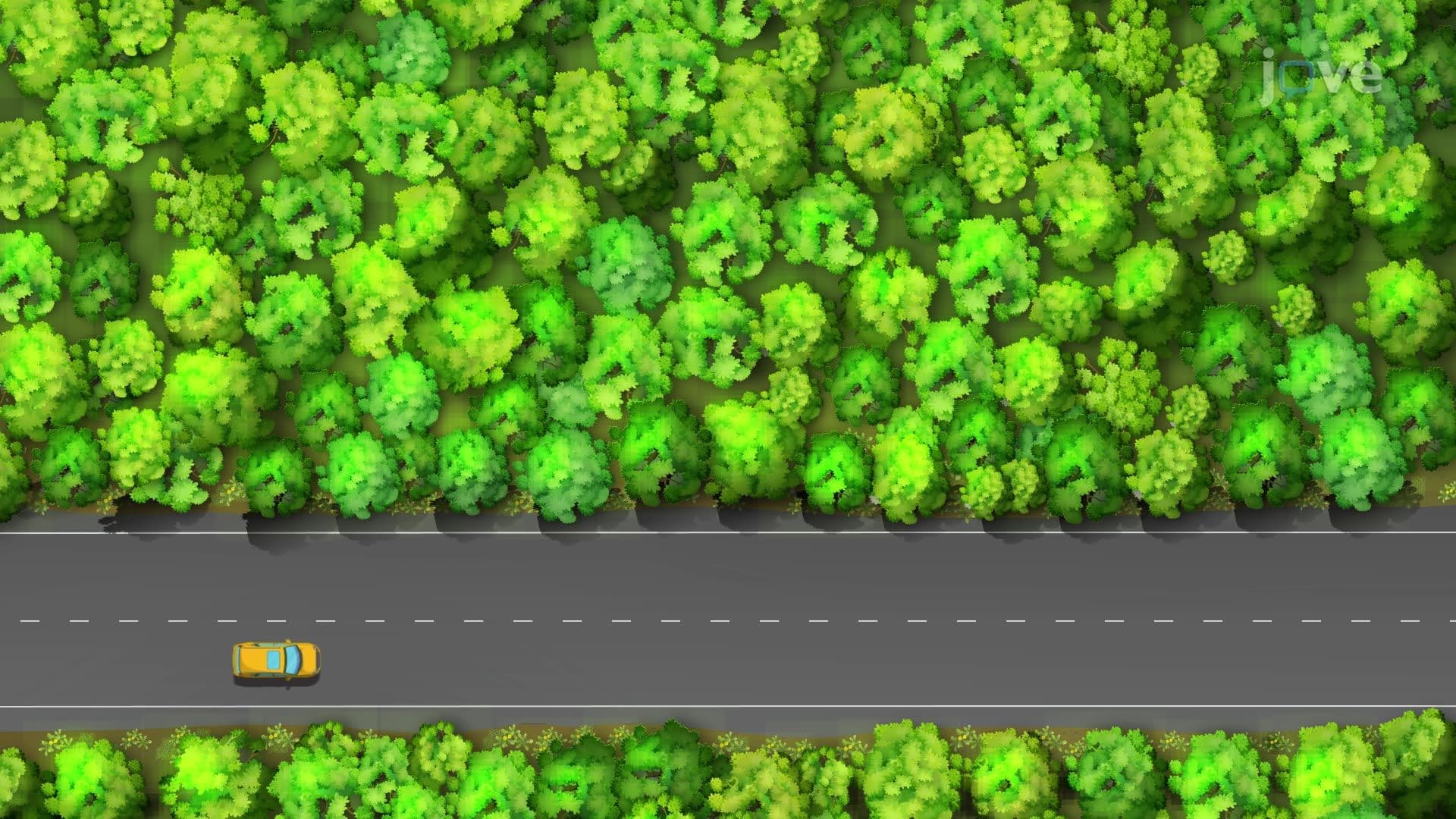
The distance problem asks a deceptively simple question: if you know how fast an object is moving at various moments in time, how do you calculate the total distance it has traveled? When velocity is constant, the answer is straightforward, distance equals velocity multiplied by time. But in real-world motion, velocity rarely stays the same. A car accelerating on a highway, a cyclist climbing a hill, or a runner pushing off the starting blocks all experience continuously changing speeds. The distance problem provides the mathematical framework to handle exactly these situations.
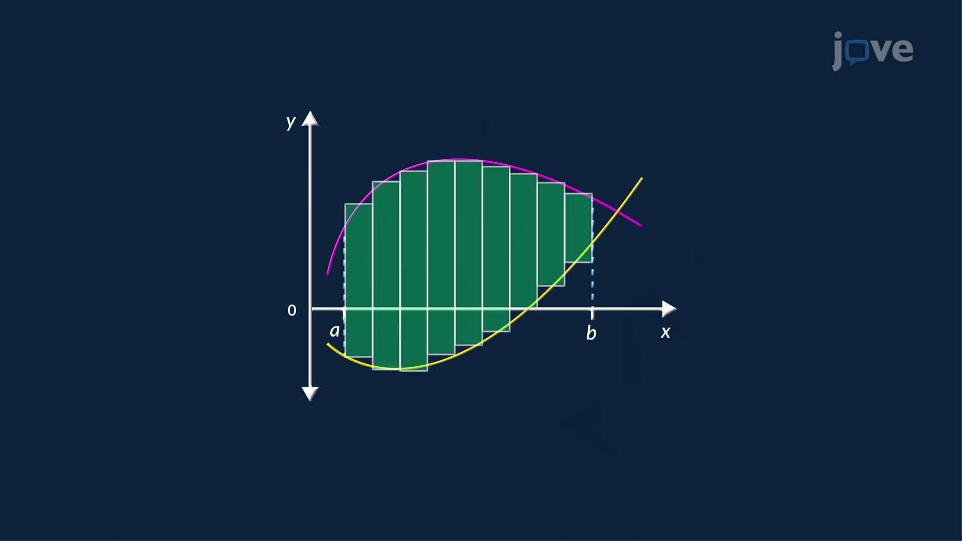
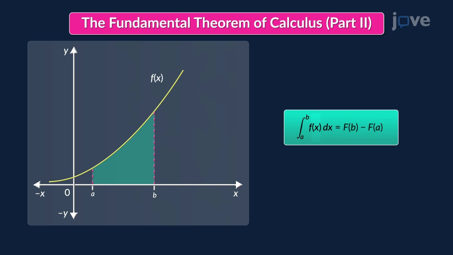
When velocity changes over time, the velocity-time graph becomes a curve rather than a flat line. The area under that curve represents the total distance traveled, but calculating it precisely requires a clever strategy. The distance problem introduces Riemann sums, a method of dividing the time interval into smaller sub-intervals and approximating the distance covered in each one using rectangle areas.
Two standard estimates are used. The lower sum uses the velocity at the left endpoint of each sub-interval, typically the slower speed at the start, giving a conservative underestimate. The upper sum uses the right endpoint velocity, typically the faster speed, producing an overestimate. The true distance lies between these two values. For example, if a runner's velocity is sampled every half-second over three seconds, the lower and upper sums might yield 10.55 meters and 13.65 meters respectively, bracketing the actual distance traveled.
The accuracy of any Riemann sum approximation depends directly on how many sub-intervals are used. With only a few wide rectangles, the approximation can be quite rough. As the number of intervals increases, and each rectangle becomes narrower, the upper and lower sums converge toward the same value. In the limit, with infinitely many infinitesimally thin rectangles, the sum becomes exact. This limiting process defines the definite integral of velocity over time, written as the integral of v(t) from t = a to t = b, and it equals the precise total distance traveled.
The distance problem is a critical topic in AP Calculus AB and BC, where students are tested on interpreting area under curves, evaluating Riemann sums, and applying the Fundamental Theorem of Calculus. College-level Calculus I courses at US universities, from community colleges to four-year institutions, use the distance problem as the primary motivation for introducing definite integrals. Students learn that antiderivatives are not just algebraic tools; they are the key to unlocking exact area calculations.
On the AP exam, free-response questions frequently present a table of velocity values and ask students to estimate distance using left, right, or midpoint Riemann sums. Understanding the distance problem deeply, not just procedurally, allows students to interpret results, justify approximations, and connect numerical methods to analytical solutions. Mastery here builds directly into broader integral topics including properties of integrals, indefinite integrals, and applications like work, area between curves, and accumulation functions.
Related Micro-courses