Growth Models with Integration: Problem Solving

• Understand how Problem Solving in Growth Models with Integration connects the rate of change of a population to its total size over time using antiderivatives.
• Identify the growth rate function G(t) and recognize it as the derivative of the biomass function B(t), setting up the integration problem correctly.
• Apply the substitution method (u-substitution) to evaluate integrals that cannot be solved by standard power rules alone.
• Analyze how initial conditions — such as a known biomass value at t = 0 — are used to solve for the constant of integration C.
• Evaluate a biomass function at a specific time value, such as t = 5, to find a population's total weight at a future date.
• Compare indefinite and definite integrals and determine which approach is most efficient when initial conditions are provided.
• Recognize how the Fundamental Theorem of Calculus connects the rate function G(t) to the accumulation function B(t) in real-world modeling.
• Explore how this integration technique extends to other growth models in biology, economics, and environmental science.

Problem Solving in Growth Models with Integration: From Rate to Total Population

When scientists or resource managers want to know *how much* of something exists — fish in a lake, bacteria in a culture, or revenue in a growing company — they often start with what they can measure most easily: the *rate* of change. Problem solving in growth models with integration is the calculus-based process of recovering a total quantity from its rate function. This technique sits at the heart of AP Calculus AB and BC, college-level Calculus I, and applied mathematics courses across the US.

What Are Growth Rate Functions and Why Do We Integrate Them?

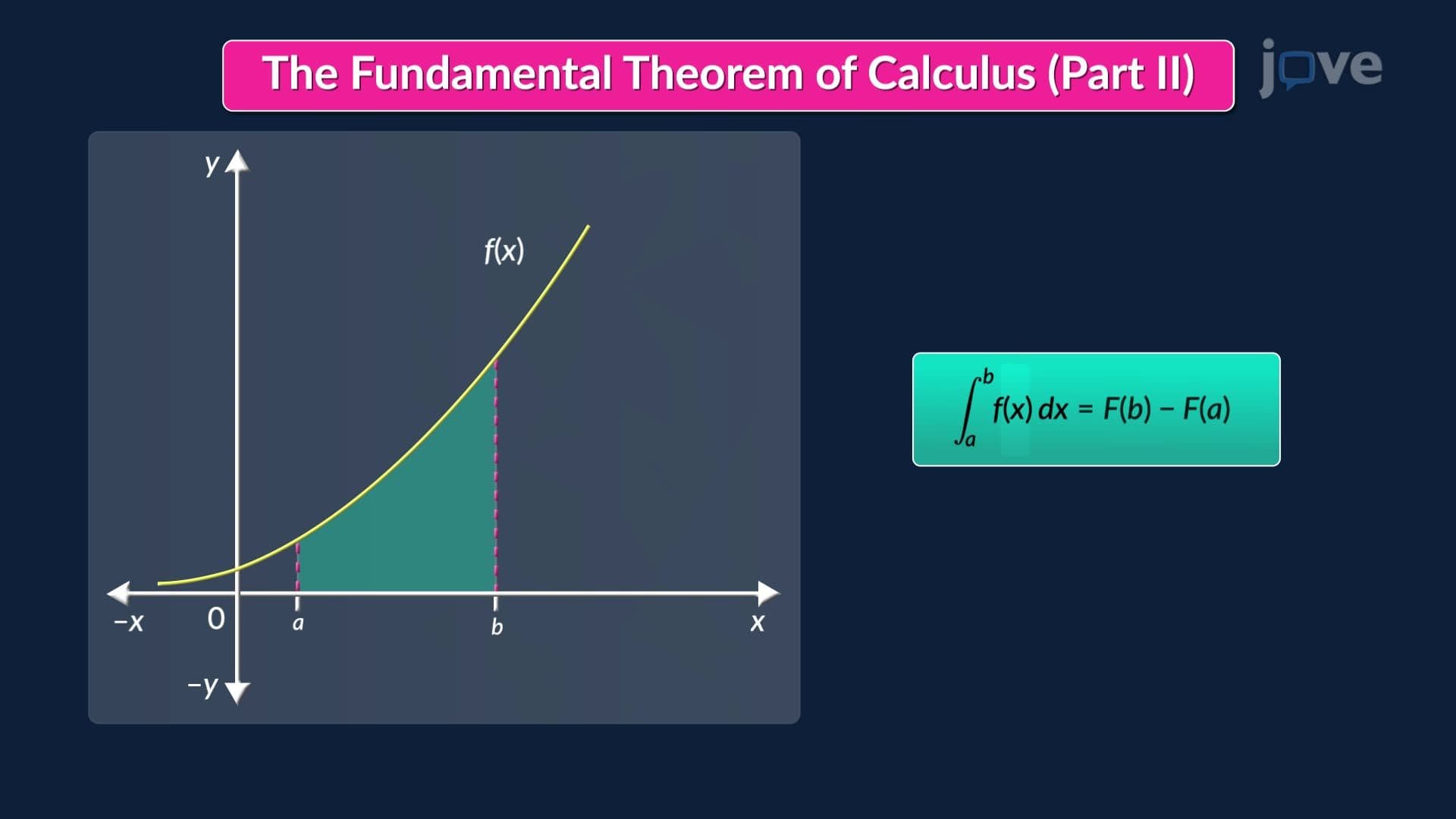
A growth rate function, often written as G(t), tells you how fast a quantity is increasing or decreasing at any given moment. In a fishery model, G(t) might represent kilograms of fish added to a lake per year. But managers need to know the *total* biomass B(t), not just the rate. Since G(t) = dB/dt — meaning G is the derivative of B — you reverse the process through integration. Finding antiderivatives is the mathematical bridge between a rate and a cumulative total. This relationship is formalized in the Fundamental Theorem of Calculus, which guarantees that if G(t) is continuous, then B(t) can be recovered by integrating G(t) with respect to t.

Using U-Substitution to Evaluate Complex Growth Integrals

Many realistic growth functions involve composite expressions that can't be integrated with a simple power rule. This is where u-substitution becomes essential. The technique works by defining a new variable u as an inner function, computing du, and rewriting the entire integral in terms of u. This simplifies the integral into a recognizable form — often a basic power or exponential integral — that is straightforward to evaluate. Once solved in terms of u, the result is translated back into the original variable t. On AP Calculus exams, u-substitution appears in roughly 20–30% of integration problems, making it one of the most heavily tested skills in the course.

Applying Initial Conditions to Find the Constant of Integration

Every indefinite integral produces a general solution containing an unknown constant C. In applied problems, this constant has a real meaning — it anchors the solution to a specific real-world scenario. Initial conditions provide a known data point, such as the fish population biomass at the year 2000 (t = 0). By substituting both the time value and the known biomass into the general equation B(t), you create a solvable algebraic equation for C. This step transforms a general antiderivative into a particular solution — the specific function that describes your unique system. This process is directly tested on AP Calculus AB free-response questions and college midterms nationwide.

Evaluating the Biomass Function at a Future Time

Once the particular solution B(t) is established, answering "What is the biomass in 2005?" is straightforward: substitute t = 5 (representing 5 years after 2000) into B(t) and simplify. This final evaluation step reinforces a key principle — calculus is not just abstract symbol manipulation. It produces numbers that answer real questions. The US Fish and Wildlife Service, for example, uses models structurally identical to this approach when setting annual harvest limits for managed fisheries. Understanding how to move from a rate function through integration to a specific numerical prediction is a foundational skill in any quantitative science or business field.